Stock Price Prediction using LSTM and its Implementation

Introduction

Have you ever wished you could predict the future, especially when it comes to your investments? While a crystal ball might be out of the question, there’s a powerful tool called an LSTM network that can analyze complex patterns in historical data, like stock prices. Unlike traditional methods, LSTMs have a special memory that allows them to remember important information for long stretches, making them ideal for navigating price movements in the ever-changing world of finance.

In this tutorial, we’ll use LSTMs and explore how a machine learning algorithm can be used to potentially predict stock prices, along with the exciting possibilities and important considerations to keep in mind.

This article was published as a part of the Data Science Blogathon.

What is LSTM?

LSTMs, are a specialized type of RNN architecture designed to tackle a specific challenge—remembering information over extended periods. These models that enhance the memory capabilities of recurrent neural networks. These networks typically hold short-term memory, utilizing earlier information for immediate tasks within the current neural network. While the neural node may not have access to a comprehensive list of past data, LSTMs are commonly employed in neural networks built on RNNs. The effectiveness of LSTMs extends across various sequence modeling problems in multiple application domains, including video, Natural Language Processing (NLP), geospatial data, and time-series analysis.

One significant issue with RNNs is the vanishing gradient problem. This issue arises due to the reuse of the same parameters in RNN blocks at each step. To address this problem, we must strive to introduce varying parameters at each time step.

Finding a balance in such scenarios is crucial. We aim to incorporate novel parameters with each step while also generalizing variable-length sequences and maintaining a constant overall number of learnable parameters. This leads us to the introduction of gated RNN cells, such as LSTM and GRU.

Gated RNN Cells and Time-Series Data

Gated cells contain internal variables known as gates. The value of each gate at a given time step is dependent on the information available at that step, including prior states. This gate value is then multiplied by different variables of interest to exert influence over them. Time-series data, which comprises a sequence of values collected at regular time intervals, enables the tracking of changes over time, be it in milliseconds, days, or years.

Traditionally, our understanding of time-series data was more static, focusing on daily temperature fluctuations or the opening and closing values of the stock market. However, with the power of LSTMs, we can now move beyond this static perspective and explore more dynamic aspects. At this point, we will transition to the coding section, where we will implement LSTM on a stocks dataset to demonstrate its capabilities in analyzing time-series data.

Best Usecases of LSTM

By selectively remembering and using past information, LSTMs can learn patterns and dependencies across long sequences. This makes them ideal for tasks like:

• Stock Market Prediction: LSTMs can analyze historical price data and past events to potentially predict future trends, considering long-term factors that might influence the price.
• Machine Translation: LSTMs can understand the context of a sentence in one language and translate it accurately into another, considering the order and relationships between words.
• Speech Recognition: LSTMs can analyze the sequence of sounds in speech and convert them into text, even when dealing with accents or background noise.

Why LSTM for Stock Price Prediction?

Here’s a detailed explanation of why LSTMs are particularly well-suited for predicting stock prices:

Challenges of Traditional Methods

• Statistical Models: Traditional statistical models like ARIMA (Autoregressive Integrated Moving Average) and linear regression assume a certain level of stationarity in the data, meaning the statistical properties (like mean and variance) remain constant over time. Stock prices, however, are non-stationary and exhibit trends and seasonality. LSTMs can handle these non-linear relationships within the data.
• Moving Averages: Simple moving averages take the average price over a defined window. While they capture recent trends, they struggle to account for long-term dependencies and sudden changes. LSTMs can learn these complex patterns better.

Overcoming Vanishing Gradients in RNNs

Standard Recurrent Neural Networks (RNNs) struggle with long sequences due to the vanishing gradient problem. In simpler terms, information from earlier time steps can become insignificantly small as it propagates through the network, making it difficult to learn long-term dependencies.

LSTM Architecture to the Rescue

LSTMs address this issue with their core component – the memory cell. This cell contains gates that control the flow of information:

• Forget Gate: Decides what information to forget from the previous cell state.
• Input Gate: Determines what new information to store in the current cell state.
• Output Gate: Controls what information from the current cell state to output.

This gating mechanism allows LSTMs to selectively remember and use past information relevant for predicting future prices, even over longer sequences.

Capturing Long-Term Dependencies

Stock prices can be influenced by events that happened months or even years ago. LSTMs can learn these long-term dependencies by selectively retaining information through the memory cell and gates.

For example, an LSTM might remember a significant economic policy change that could have a long-term impact on a company’s stock price.

In essence, LSTMs provide a powerful tool for building predictive model for time series data like stock prices by overcoming the limitations of traditional methods and standard RNNs. They can capture complex patterns and long-term dependencies within the data, making them a valuable approach for stock forecast, although with inherent limitations and the ever-present volatility of the market.

Implementation of LSTM on Stocks Data in Python

This section explores a powerful methodology for stock price prediction using machine learning model. Long Short-Term Memory (LSTM) networks implemented in Python. Here’s a breakdown of the key steps:

Dataset

We will be using Learning-Pandas-Second-Edition dataset.

Reading Stock Market Data

gstock_data = pd.read_csv('data.csv')
gstock_data .head()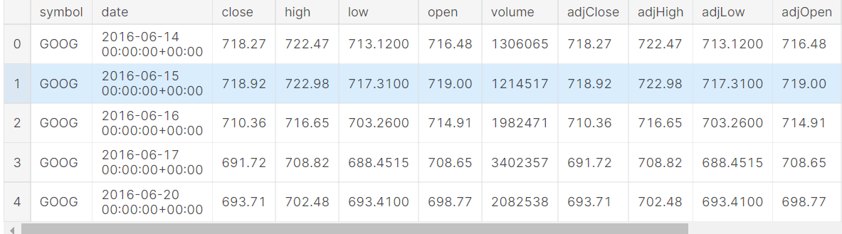

Exploring Dataset

The dataset contains 14 columns associated with time series like the date and the different variables like close, high, low and volume. We will use opening and closing values for our experimentation of time series with LSTM.

gstock_data = gstock_data [['date','open','close']] 
gstock_data ['date'] = pd.<a onclick="parent.postMessage({'referent':'.pandas.to_datetime'}, '*')">to_datetime(gstock_data ['date'].apply(lambda x: x.split()[0])) 
gstock_data .set_index('date',drop=True,inplace=True) 
gstock_data .head()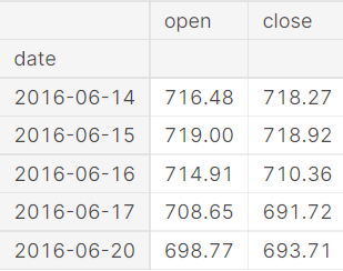

In this section, we’ve performed feature extraction by isolating the date component from the comprehensive date variable. This isolation allows us to focus specifically on the date information. To gain insights into our data, we can employ Matplotlib to visualize the extracted information. In this case, we’re interested in understanding how the price values behave over time.

When creating the price-date graph, we’ve chosen specific colors to represent different variables. The ‘open’ price values are depicted in green, offering a visual representation of the initial price for each date. On the other hand, the ‘closing’ price values are shown in red, indicating the final price for each corresponding date. This color coding makes it easier to distinguish between the opening and closing prices, providing a clear visualization of the price movement over the given timeframe.

fg, ax =plt.<a onclick="parent.postMessage({'referent':'.matplotlib.pyplot.subplots'}, '*')">subplots(1,2,figsize=(20,7))
ax[0].plot(gstock_data ['open'],label='Open',color='green')
ax[0].set_xlabel('Date',size=15)
ax[0].set_ylabel('Price',size=15)
ax[0].legend()
ax[1].plot(gstock_data ['close'],label='Close',color='red')
ax[1].set_xlabel('Date',size=15)
ax[1].set_ylabel('Price',size=15)
ax[1].legend()
fg.show()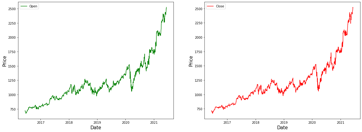

Data Pre-processing

We must pre-process this data before applying stock price using LSTM. Transform the values in our data with help of the fit_transform function. Min-max scaler is used for scaling the data so that we can bring all the price values to a common scale. We then use 80 % data for training and the rest 20% for testing and assign them to separate variables.

from sklearn.preprocessing import MinMaxScaler
Ms = MinMaxScaler()
gstock_data [gstock_data .columns] = Ms.fit_transform(gstock_data )

training_size = round(len(gstock_data ) * 0.80)

train_data = gstock_data [:training_size]
test_data  = gstock_data [training_size:]

Splitting Data for Training

A function is created so that we can create the sequence for training and testing.

def create_sequence(<a onclick="parent.postMessage({'referent':'.kaggle.usercode.22406117.81090952.create_sequence..dataset'}, '*')">dataset):
  <a onclick="parent.postMessage({'referent':'.kaggle.usercode.22406117.81090952.create_sequence..sequences'}, '*')">sequences = []
  <a onclick="parent.postMessage({'referent':'.kaggle.usercode.22406117.81090952.create_sequence..labels'}, '*')">labels = []

  <a onclick="parent.postMessage({'referent':'.kaggle.usercode.22406117.81090952.create_sequence..start_idx'}, '*')">start_idx = 0

  for <a onclick="parent.postMessage({'referent':'.kaggle.usercode.22406117.81090952.create_sequence..stop_idx'}, '*')">stop_idx in range(50,len(<a onclick="parent.postMessage({'referent':'.kaggle.usercode.22406117.81090952.create_sequence..dataset'}, '*')">dataset)): 
    <a onclick="parent.postMessage({'referent':'.kaggle.usercode.22406117.81090952.create_sequence..sequences'}, '*')">sequences.append(<a onclick="parent.postMessage({'referent':'.kaggle.usercode.22406117.81090952.create_sequence..dataset'}, '*')">dataset.iloc[<a onclick="parent.postMessage({'referent':'.kaggle.usercode.22406117.81090952.create_sequence..start_idx'}, '*')">start_idx:<a onclick="parent.postMessage({'referent':'.kaggle.usercode.22406117.81090952.create_sequence..stop_idx'}, '*')">stop_idx])
    <a onclick="parent.postMessage({'referent':'.kaggle.usercode.22406117.81090952.create_sequence..labels'}, '*')">labels.append(<a onclick="parent.postMessage({'referent':'.kaggle.usercode.22406117.81090952.create_sequence..dataset'}, '*')">dataset.iloc[<a onclick="parent.postMessage({'referent':'.kaggle.usercode.22406117.81090952.create_sequence..stop_idx'}, '*')">stop_idx])
    <a onclick="parent.postMessage({'referent':'.kaggle.usercode.22406117.81090952.create_sequence..start_idx'}, '*')">start_idx += 1
  return (np.<a onclick="parent.postMessage({'referent':'.numpy.array'}, '*')">array(<a onclick="parent.postMessage({'referent':'.kaggle.usercode.22406117.81090952.create_sequence..sequences'}, '*')">sequences),np.<a onclick="parent.postMessage({'referent':'.numpy.array'}, '*')">array(<a onclick="parent.postMessage({'referent':'.kaggle.usercode.22406117.81090952.create_sequence..labels'}, '*')">labels))

train_seq, train_label = create_sequence(train_data)
test_seq, test_label = create_sequence(test_data)

Implementation of our LSTM Model

In the next step, we create our LSTM model.  In this article, we will use the Sequential model imported from Keras and required libraries are imported.

from keras.models import Sequential
from keras.layers import Dense, Dropout, LSTM, Bidirectional

We use two LSTM layers in our model and implement drop out in between for regularization. The number of units assigned in the LSTM parameter is fifty. with a dropout of 10 %. Mean squared error is the loss function for optimizing the problem with adam optimizer. Mean absolute error is the metric used in our LSTM network as it is associated with time-series data.

model = Sequential()
model.add(LSTM(units=50, return_sequences=True, input_shape = (train_seq.shape[1], train_seq.shape[2])))

model.add(Dropout(0.1)) 
model.add(LSTM(units=50))

model.add(Dense(2))

model.compile(loss='mean_squared_error', optimizer='adam', metrics=['mean_absolute_error'])

model.summary()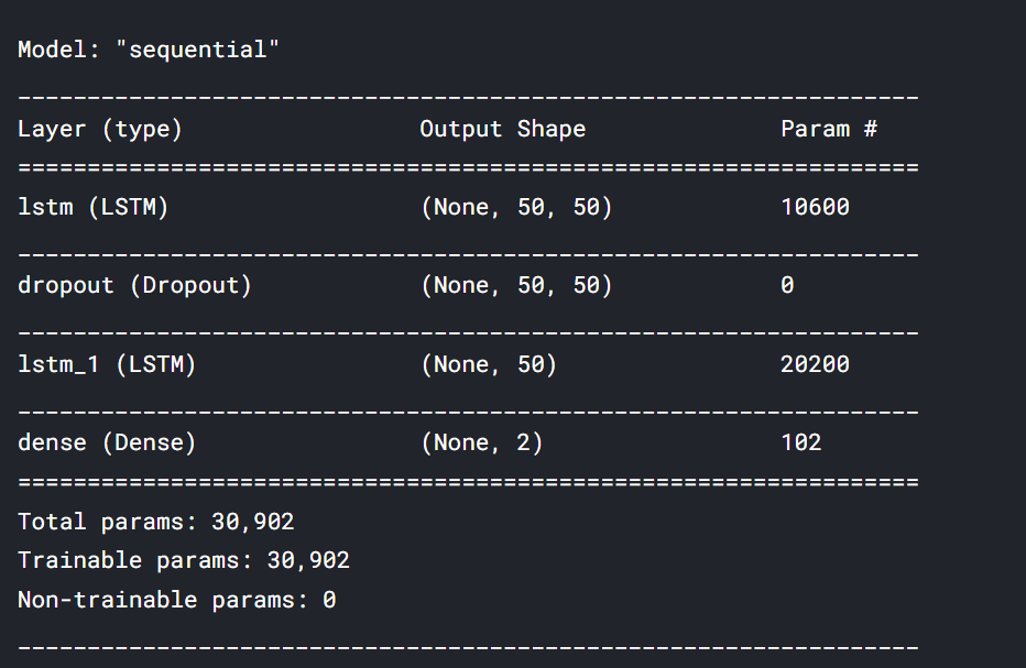

model.fit(train_seq, train_label, epochs=80,validation_data=(test_seq, test_label), verbose=1)
test_predicted = model.predict(test_seq)
test_inverse_predicted = MMS.inverse_transform(test_predicted)

Visualization

After fitting the data with our model we use it for prediction. We must use inverse transformation to get back the original value with the transformed function. Now we can use this data to visualize the short-term stock price change predictions.

# Merging actual and predicted data for better visualization
gs_slic_data = pd.concat([gstock_data .iloc[-202:].copy(),pd.DataFrame(test_inverse_predicted,columns=['open_predicted','close_predicted'],index=gstock_data .iloc[-202:].index)], axis=1)

gs_slic_data[['open','close']] = MMS.inverse_transform(gs_slic_data[['open','close']])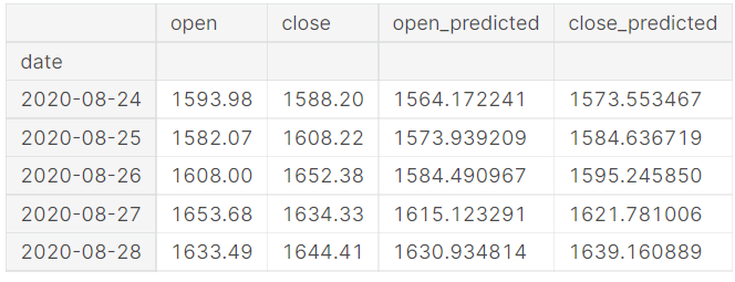

gs_slic_data[['open','open_predicted']].plot(figsize=(10,6))
plt.<a onclick="parent.postMessage({'referent':'.matplotlib.pyplot.xticks'}, '*')">xticks(rotation=45)
plt.<a onclick="parent.postMessage({'referent':'.matplotlib.pyplot.xlabel'}, '*')">xlabel('Date',size=15)
plt.<a onclick="parent.postMessage({'referent':'.matplotlib.pyplot.ylabel'}, '*')">ylabel('Stock Price',size=15)
plt.<a onclick="parent.postMessage({'referent':'.matplotlib.pyplot.title'}, '*')">title('Actual vs Predicted for open price',size=15)
plt.<a onclick="parent.postMessage({'referent':'.matplotlib.pyplot.show'}, '*')">show()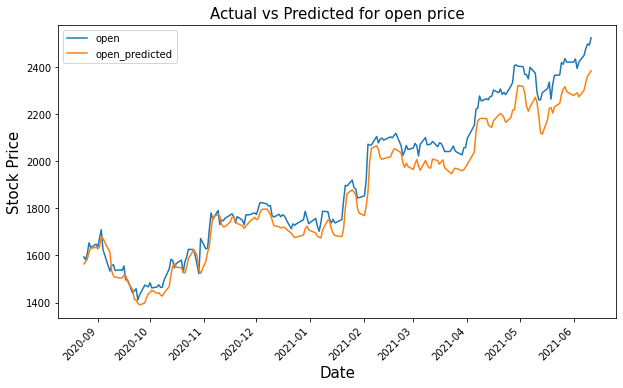

gs_slic_data[['close','close_predicted']].plot(figsize=(10,6))
plt.<a onclick="parent.postMessage({'referent':'.matplotlib.pyplot.xticks'}, '*')">xticks(rotation=45)
plt.<a onclick="parent.postMessage({'referent':'.matplotlib.pyplot.xlabel'}, '*')">xlabel('Date',size=15)
plt.<a onclick="parent.postMessage({'referent':'.matplotlib.pyplot.ylabel'}, '*')">ylabel('Stock Price',size=15)
plt.<a onclick="parent.postMessage({'referent':'.matplotlib.pyplot.title'}, '*')">title('Actual vs Predicted for close price',size=15)
plt.<a onclick="parent.postMessage({'referent':'.matplotlib.pyplot.show'}, '*')">show()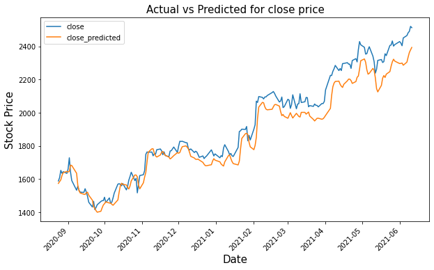

Challenges

Even though LSTMs offer advantages for predicting stock market prices, there are still challenges to consider:

• Data Quality and Noise: Stock prices are influenced by a multitude of factors, many of which are unpredictable (e.g., news events, social media sentiment). LSTMs might struggle to differentiate between relevant patterns and random noise in the data, potentially leading to inaccurate predictions.
• Limited Historical Data: The effectiveness of LSTMs depends on the quality and quantity of historical data available. For newer companies or less liquid stocks, there might not be enough data to train the model effectively, limiting its ability to capture long-term trends.
• Non-Linear Relationships: While LSTMs can handle complex relationships, the stock market can exhibit sudden shifts and non-linear behavior due to unforeseen events. The model might not be able to perfectly capture these unpredictable fluctuations.
• Overfitting and Generalizability: There’s a risk of the model overfitting the training data, performing well on historical data but failing to generalize to unseen future patterns. Careful hyperparameter tuning and validation techniques are crucial to ensure the model can learn generalizable insights.
• Self-Fulfilling Prophecies: If a large number of investors rely on LSTM predictions, their collective actions could influence the market in a way that aligns with the prediction, creating a self-fulfilling prophecy. This highlights the importance of using these predictions as a potential guide, not a guaranteed outcome.

Despite these challenges, LSTM algorithm remain a good predictor for analyzing stock price data. By understanding these limitations and implementing best practices, you can leverage the strengths of LSTMs to gain valuable insights into the financial markets.

Disclaimer

This blog post explores the potential of Long Short-Term Memory networks (LSTMs) as a dynamic tool for stock price prediction. While LSTMs present a robust method for analyzing and forecasting stock prices, this blog underscores the importance of not exclusively depending on them for investment strategies. Proactive steps towards informed decision-making include conducting independent research, utilizing a range of analytical tools, and seeking guidance from experienced financial advisors.

Conclusion

LSTMs offer a glimpse into the future of share price prediction by analyzing historical data and capturing long-term patterns. However, the stock market’s inherent volatility and limitations like data quality and non-linear relationships prevent perfect forecasts.

Despite these challenges, LSTMs remain a valuable tool for financial analysis. By understanding their strengths and weaknesses with technical analysis, you can leverage them and include them into your trading strategy to gain valuable market insights and make informed investment decisions.

Reference:

• https://the-learning-machine.com/article/dl/long-short-term-memory
• https://www.kaggle.com/amarsharma768/stock-price-prediction-using-lstm/notebook

The media shown in this article is not owned by Analytics Vidhya and are used at the Author’s discretion.  

Frequently Asked Questions

Siddharth M 02 Jun 2024