Logo:
Logo:  Areas Served:
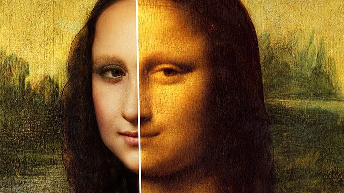
Processing Monalisa: Image Processing with Scikit-image.
Last Updated on January 30, 2024 by Editorial Team
Author(s): Rakesh M K
Originally published on Towards AI.
Scikit-image.
Scikit-image is an open-source Python library for image processing that offers various algorithms for color conversion, filtering, thresholding segmentation, denoising, etc. On this page, we will see some of them applied to the famous painting ‘Monalisa’ done by the Italian polymath Leonardo da Vinci in the early 16th century.
Install Scikit-image.
Scikit-image can be installed using pip or with conda, as given below.
!pip install scikit-image
conda install -c conda-forge scikit-image
Import Monalisa
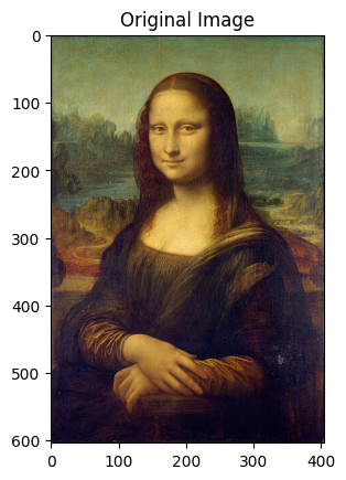
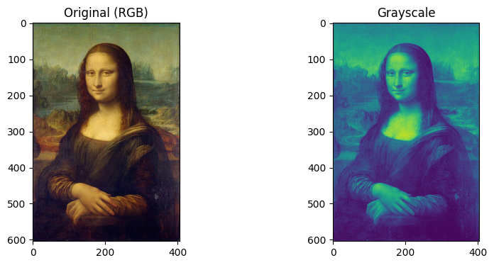
The image is imported using imageio library and displayed using matplotlib. The shape of the image is 604x405x3 (height, width, channels). The 3 channels correspond to three color channels, which implies that it is an RGB image.
import skimage
import imageio
import matplotlib.pyplot as plt

imagePath = 'monalisa.JPG' # path to image
monalisa = imageio.imread(imagePath)
plt.imshow(monalisa)
plt.title('Original Image')
plt.show()print(monalisa.shape) # checking shape of the image
(604, 405, 3)
RGB to Grayscale
In grayscale conversion, the number of channels will be reduced to 1. Generally, the grayscale values range from 1 to 255 but scikit-image outputs normalized values in a range [0,1] for numerical stability. (Normalization: each pixel value/255). The conversion can be done with the function rgb2gray by importing from skimage.color.
from skimage.color import rgb2gray

monalisaGray = rgb2gray(monalisa)
colorSpace = ['Original (RGB)', 'Grayscale']
images = [monalisa, monalisaGray]
fig, axes = plt.subplots(1, len(colorSpace), figsize= (10,4))

for idx, s in enumerate(colorSpace):
 axes[idx].imshow(images[idx])
 axes[idx].set_title(f'{colorSpace[idx]}')
plt.show()
The change in shape can be seen in the snippet below.
monalisa.shape, monalisaGray.shape(604, 405, 3)), ((604, 405)
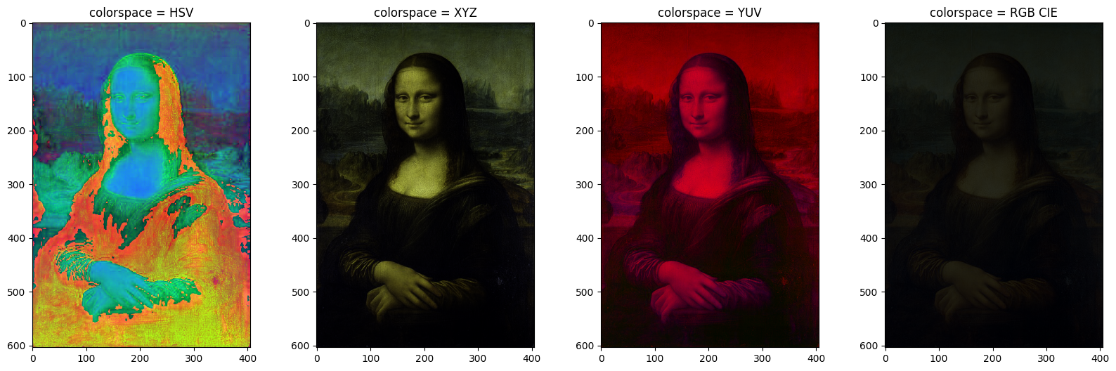
Color conversion.
Transforming the color representation of an image from one color space to another is called color conversion. Some of the color spaces are 'HSV', 'XYZ', 'YUV', 'RGB CIE' etc. The below snippet converts the original image to listed color spaces as in the figure with use of convert_colorspace the function. To read more about color spaces and their uses elaborately, visit the wiki page List of color spaces and their uses — Wikipedia.
from skimage.color import convert_colorspace '''create list of required color spaces.'''
colorSpace = ['HSV', 'XYZ', 'YUV', 'RGB CIE']fig, axes = plt.subplots(1, len(colorSpace), figsize= (20,6))

for idx, s in enumerate(colorSpace):
 monalisaColor = convert_colorspace(monalisa ,'RGB', s)
 axes[idx].imshow(monalisaColor)
 axes[idx].set_title(f'colorspace = {s}')
plt.show()
Alternatively, the same can be done using functionrgb2hsv, rgb2xyz, rgb2yuv etc. by importing these from skimage.color . e.g. image = rgb2hsv(monalisa).
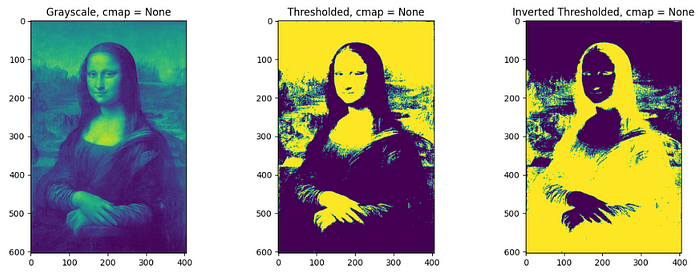
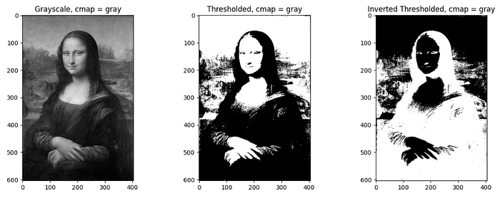
Thresholding and Inverted thresholding
Thresholding classifies pixel values with respect to a specified threshold value. Pixel value above the threshold will be converted to 1 and below as 0 in thresholding whereas in opposite manner in inverse thresholding. It is straightforward to do thresholding on grayscale images, but for RGB images, thresholding on each channel should be done separately and combined later. A threshold of 0.3 (since the grayscale obtained by the image is normalized) is used for the processing of the image in the below code.
Different color mapping can be used to display the converted image by setting cmap inside plt.imshow() for different visual experiences. e.g. plt.imshow(image, cmap = ‘jet’). To check different available color mappings in matplotlib, visit Choosing Colormaps — Matplotlib 3.8.2 documentation.
th = 0.3 # set threshold value

img1 = monalisa >= th # thresholding
img2 = monalisa <= th # inverted thresholding

img = [monalisa, img1, img2]
title = ['Original', 'Thresholded', 'Inverted Thresholded']

fig, axes = plt.subplots(1, len(title), figsize= (20,6))
for idx, s in enumerate(title):
 axes[idx].imshow(img[idx])
 axes[idx].set_title(f'colorspace = {s}')
plt.show()
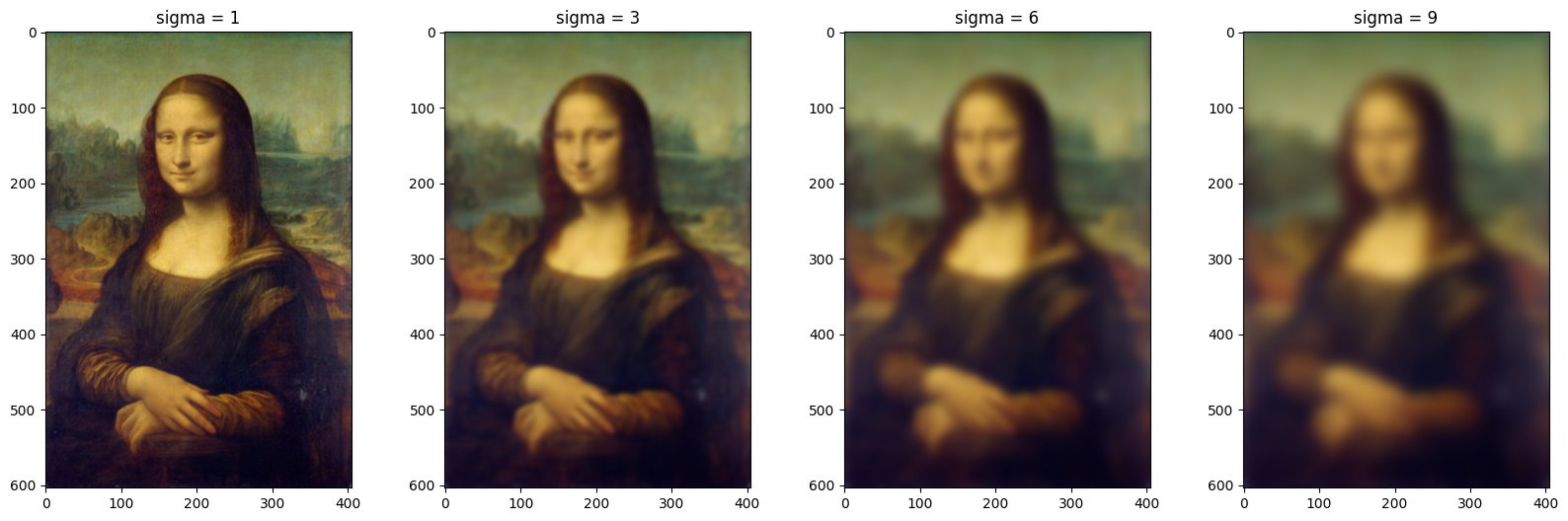
Filtering-1: Gaussian
Gaussian filtering is a type of low-pass filter that is mainly used to introduce noise or blur in the image(smoothening). Parameter sigma is the standard deviation of the Gaussian distribution, which determines the spread of the Gaussian function. Once sigma increases, the smoothening or noise introduced in the image increases, as you see in the below plot.
from skimage.filters import gaussian'''set list of sigma values.'''
sigma = [1, 3, 6, 9]

fig, axes = plt.subplots(1, len(sigma), figsize= (20,6))
for idx, s in enumerate(sigma):
 axes[idx].imshow(gaussian(monalisa , sigma = s))
 axes[idx].set_title(f'sigma = {s}')
plt.show()
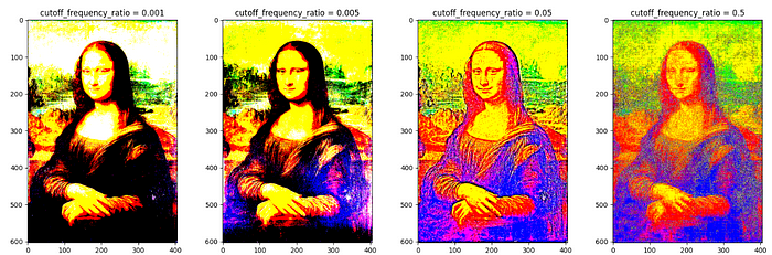
Filtering-2: Butterworth
Butterworth filter is a frequency domain filter that is used to enhance the images. It works by passing certain frequencies and attenuating others. order and cutoff_frequency_ratio are the main parameters of the filter. The parameter order can be understood as the number of times the filtering is applied to the image. Higher order leads to rapid increases in attenuation beyond cutoff frequency.
Butterworth filtering with various values of cutoff_frequency_ratio :
from skimage.filters import butterworth'''create a list of cutoff frequency ratio.'''
f_cutoff = [.001,.005,.05, .5]fig, axes = plt.subplots(1, len(f_cutoff), figsize= (20,6))
for idx, s in enumerate(f_cutoff):
 axes[idx].imshow(butterworth(monalisa , cutoff_frequency_ratio = f_cutoff[idx]))
 axes[idx].set_title(f'cutoff_frequency_ratio = {f_cutoff[idx]}')
plt.show()
Butterworth filtering with various value of order = [1,2,3,4]keeping cutoff_frequency_ratio = 0.5 .
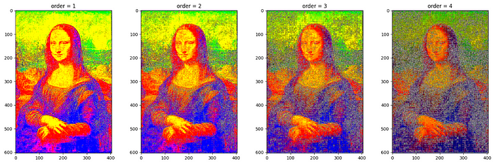
order.For more filters on RGB images (Laplace, Median etc.), refer to skimage.filters — skimage 0.22.0 documentation (scikit-image.org).
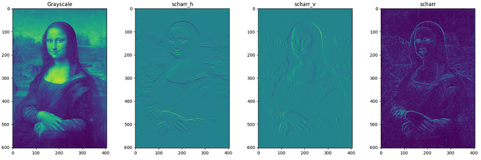
Filtering-3: Farid, Scharr, Prewitt, Sobel, Roberts (for bimodal Images).
These filters are used for edge detection of bimodal (grayscale) images. Filters can be applied along vertical and horizontal axes also. The filtered images represent the gradient of the original image along each axis where gradient is the rate of change of pixel intensity. The below code written for farid filters can be applied to sobel, prewitt and scharr filters (Only filtered images included in this page). For roberts filter, it is roberts_neg_diag ,roberts_pos_diag instead of horizontal and vertical where neg and pos denote the diagonal direction of kernel.
Note: The below code can be extended to all other filters. Only filter outputs are included.
from skimage.filters import farid, farid_h , farid_v

monalisaF = farid(monalisaGray)
monalisaFh = farid_h(monalisaGray)
monalisaFv = farid_v(monalisaGray)


F = ['Grayscale','farid_h', 'farid_v', 'farid']
I = [monalisaGray, monalisaF , monalisaFh, monalisaFv]
fig, axes = plt.subplots(1, len(I), figsize=(20,6))

for idx, img in enumerate(I):
 axes[idx].imshow(img,cmap = 'gray')
 axes[idx].set_title(f'filter: {F[idx]}')
plt.show()


Even if the output of all these filters looks same, the pixel values differ in value. Checking just one element in the filtered image pixel values of all filters as below it can be clearly understood.
print(monalisaSob[1][1], monalisaS[1][1],monalisaR[1][1], monalisaP[1][1], monalisaF[1][1])0.05072484484173028 0.05344169652064987 0.0697070304160717 0.04828679324051692 0.017526469293676204
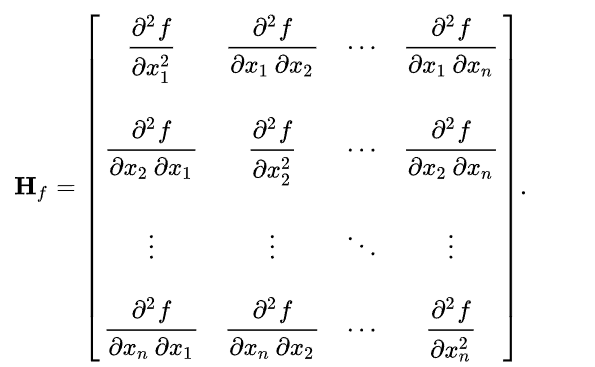
Filtering-4: Hessian, Frangi.
Frangi and Hessian filters have application beyond edge detection and and are mainly used in medical image processing. Both of these filters make use of properties of Hessian matrix which is a square matrix of second order partial derivatives.
Hessian filters use the Hessian matrix as kernel, whereas Frangi filters use eigenvalues of a Hessian matrix. Frangi filters highlight the tubular structures and curvatures in the image and are specially designed for medical images such that they can detect blood vessels. Hessian filters are useful for detecting structures based on their local shape, which makes them useful for the segmentation of medical images.
from skimage.filters import frangi , hessian

F = ['Grayscale','frangi', 'hessian', 'hessian(on RGB)']
I = [monalisaGray,frangi(monalisaGray), hessian(monalisa), hessian(monalisaGray),]
fig, axes = plt.subplots(1, len(I), figsize=(20,6))

for idx, img in enumerate(I):
 axes[idx].imshow(img, cmap = 'gray')
 axes[idx].set_title(f'filter = {F[idx]}')
plt.show()
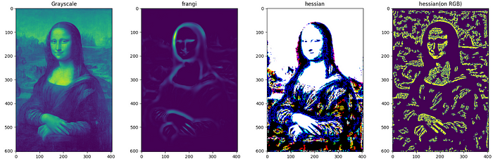
While it can be used with both grayscale and RGB images, this filter works well with grayscale images.
Filtering on RGB images.
The filters which we used for edge detection of bimodal images (scharr, sobel, farid, roberts etc.) can be used for RGB images with the help of decorators as below. The filter acts on each channel, and later, the filtered values of all channels are combined. An example of the Sobel filter is given below.
To read more about Python decorators visit: https://realpython.com/primer-on-python-decorators/
from skimage.color import adapt_rgb, each_channel, hsv_value
from skimage.exposure import rescale_intensity
from skimage import data, filters

@adapt_rgb(each_channel)
def sobelEach(image):
 return filters.sobel(image)

@adapt_rgb(hsv_value)
def sobelHSV(image):
 return filters.sobel(image)

img1 = rescale_intensity(1- scharrEach(monalisa))
img2 = rescale_intensity(1- scharrHSV(monalisa))


I = [monalisa, img1, img2]
F = ['original',' sobel (each channel)', 'sobel (HSV)']

fig, axes = plt.subplots(1, len(I), figsize=(20,6))

for idx, img in enumerate(I):
 axes[idx].imshow(img,cmap = 'gray')
 axes[idx].set_title(f'filter = {F[idx]}')
plt.show()

Conclusion
We have seen some of the features of Scikit-image on this page, mainly filters. The library offers many more algorithms, such as drawing shapes, thresholding, segmentation, image restoration, denoising, and much more. Those can be explored from the page scikit-image: Image processing in Python — scikit-image.
References
U+2709️ [email protected]
Join thousands of data leaders on the AI newsletter. Join over 80,000 subscribers and keep up to date with the latest developments in AI. From research to projects and ideas. If you are building an AI startup, an AI-related product, or a service, we invite you to consider becoming a sponsor.
Published via Towards AI
Related posts
Popular posts

 for 2021")


Updates

Recent Posts