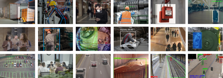
Whether you’re building a consumer app to recognize plant species or an enterprise tool to monitor office security camera footage, you are going to need to build a Machine Learning (ML) model to provide the core functionality. Today, building an ML model is easier than ever before using frameworks like Tensorflow. However, it’s still important to follow a methodical workflow to avoid building a model with poor performance or inherent bias.
Building a machine learning model consists of 7 high-level steps:
1. Problem Identification
2. Dataset Creation
3. Model Selection
4. Model Training
5. Model Assessment
6. Model Optimization
7. Model Deployment and Maintenance
In this article, we’ll break down what’s involved in each step, with a focus on supervised learning models.
About us: Viso Suite is the computer vision infrastructure for enterprises.
Step 1: Identify a Problem for the Model To Solve
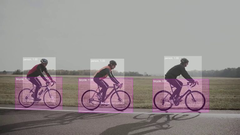
To build a model, we first need to identify the specific problem that our model should solve. The problem could be reading pharmaceutical labels using images from a lab camera, to identify threats from a school security camera feed or anything else.
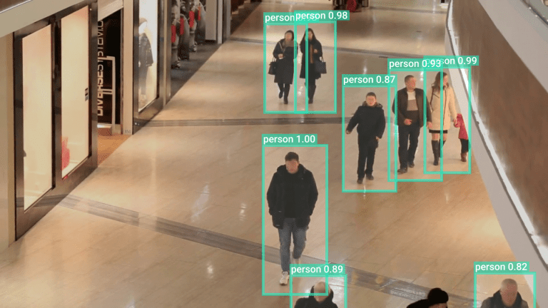
The example image below is from a model that was built to identify and segment people within images.

Step 2: Create a Dataset for Model Training & Testing
Before we can train a machine learning model, we need to have data on which to train.
We generally don’t want a pile of unorganized data. Typically, we need to first gather data, then clean the data, and finally engineer specific data features that we anticipate will be most relevant to the problem we identified in Step 1.
Data gathering
There are four possible approaches to data gathering. Each relies on different data sources.
The first approach is to construct a proprietary dataset. For example, if we want to train a machine learning model to read labels at a pharmacy, then constructing a proprietary dataset would mean gathering tens of thousands to potentially tens of millions of images of labels and having humans create a CSV file associating the file name of each image with the text of the label shown in that image.
As you’d expect, this can be very time-consuming and very expensive. However, if our intended use case is very novel (for example, diagnosing automotive issues for BMWs using images of the engine block), then constructing a proprietary dataset may be necessary. This approach also removes the risk of systematic bias in data collected from third parties. That can save data scientists a lot of time since data preparation and cleaning can be very time-consuming.
The second approach is to use one or more existing datasets. This is usually much cheaper and more scalable than the first approach. However, the collected data can also be of lower quality.
The third approach is to combine one or more existing datasets with a smaller proprietary dataset. For example, if we want to train a machine learning model to read pharmaceutical pill bottle labels, we might combine a large general dataset of images with text with a smaller dataset of labeled pill bottle images.
The fourth approach is to create synthetic data. This is an advanced technique that should be used with caution since using synthetic data incorrectly can lead to bad models that perform fantastically on assessments but terribly in the real world.
Data cleaning
If we gather data using the second or third approach described above, then it’s likely that there will be some amount of corrupted, mislabeled, incorrectly formatted, duplicate, or incomplete data that was included in the third-party datasets. By the principle of garbage in, and garbage out, we need to clean up those data issues before feeding the data into our model.
Exploratory data analysis & feature engineering
If you’ve ever taken a calculus class, you may remember doing a “change of variables” to solve certain problems. For example, changing from Euclidean x-y coordinates to polar r-theta coordinates. Changing variables can sometimes make it much easier to solve a problem (just try writing down an integral for the area of a circle in Euclidean vs polar coordinates).
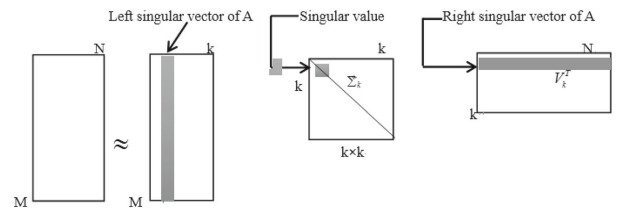
Feature engineering is just a change of variables that makes it easier for our model to identify meaningful patterns than would be the case using the raw data. It can also help reduce the dimensionality of the input which can help to avoid overfitting in situations where we don’t have as much training data as we would like.
How do we perform feature engineering? It often helps to do some exploratory data science.
Try running some basic statistical analyses on your data. Generate some plots of different subsets of variables. Look for patterns.
For example, if your model is going to be trained on audio data, you might want to do a Fourier transform of your data and use the Fourier components as features.
Step 3: Select a Model Architecture
Now that we have a large enough dataset that has been cleaned and feature-engineered, we need to choose what type of model to use.
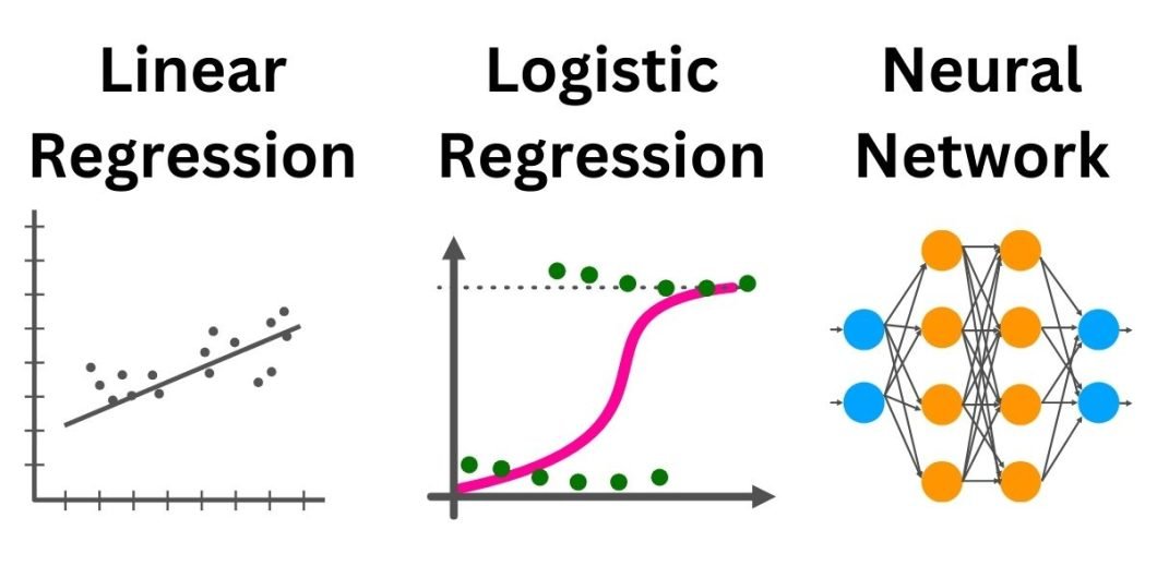
Some common types of machine learning algorithms include:
- Regression models (e.g. linear regression, logistic regression, Lasso regression, and ridge regression)
- Convolutional neural networks (these are commonly used for computer vision applications)
- Recurrent neural networks (these are used on text and genomic data)
- Transformers (these were originally developed for text data but have since also been adapted to computer vision applications)
Ultimately, the type of model you select will depend on (1) the type of data that will be input into the model (e.g. text vs images) and (2) the desired output (e.g. a binary classification or a bounding box for an image).
Step 4: Train the Model
Once we have our selected model and our cleaned dataset with engineered features, we are ready to start training our AI model.
Loss functions
To start, we need to choose a loss function. The purpose of the loss function is to tell us how far apart our expected and predicted values are on every input to our model. The model will then be “trained” by repeatedly updating the model parameters to minimize the loss function across our training dataset.
The most common loss function is the Mean Squared Error (also called the L2 loss). The L2 loss is a smooth function which means it can be differentiated without any issues. That makes it easy to use gradient descent to minimize the loss function during model training.
Another common loss function is the Mean Absolute Error (also called the L1 loss). The L1 loss is not a smooth function, which means it is harder to use gradient descent to train the model. However, the L1 loss function is less sensitive to outliers than the L2 loss function. That can sometimes make it worthwhile to use the L1 loss function to make the model training more robust.
Training data
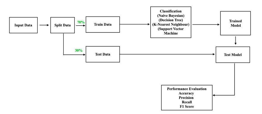
After we choose our loss function, we need to decide how much of our data to use for training and how much to reserve for testing. We don’t want to train and test on the same data otherwise we run the risk of over-fitting our model and overestimating the model’s performance based on a statistically flawed test.
It’s common practice to use 70-80% of your data for training and keep the remaining 20-30% for testing.
Training procedure
The high-level training procedure for building an AI model is pretty much the same regardless of the type of model. Gradient descent is used to find a local minimum of the loss function averaged across the training dataset.
For neural networks, gradient descent is accomplished through a technique called backpropagation. You can read more about the theory of backpropagation here. However, it’s easy to perform backpropagation in practice without knowing much theory by using libraries like Tensorflow or Pytorch.
Step 5: Model Assessment
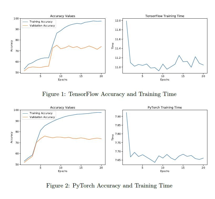
Now that we finished training our machine learning model, we need to assess its performance.
Model testing
The first step of model assessment is model testing (also called model validation).
This is where we calculate the average value of the loss function across the data we set aside for testing. If the average loss on the testing data is similar to the average loss on the training data, then our model is good. However, if the average loss on the testing data is substantially higher than the average loss on the training data, then there is a problem either with our data or with our model’s ability to adequately extrapolate patterns from the data.
Cross-validation
The choice of which portion of our data to use as the training set and which to use as the testing set is an arbitrary one, but we don’t want our model’s predictions to be arbitrary. Cross-validation is a technique to test how dependent our model performance is on the particular way that we choose to slice up the data. Successful cross-validation gives us confidence that our model is actually generalizable to the real world.
Cross-validation is easy to perform. We start by bucketing our data into chunks. We can use any number of chunks, but 10 is common. Then, we re-train and re-test our model using different sets of chunks.
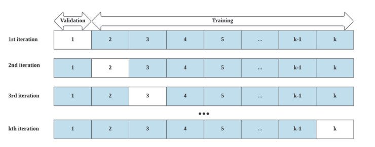
For example, suppose we bucket our data into 10 chunks and use 70% of our data for testing. Then cross-validation might look like this:
- Scenario 1: Train on chunks 1-7 and test on chunks 8-10.
- Scenario 2: Train on chunks 4-10 and test on chunks 1-3.
- Scenario 3: Train on chunks 1-3 and 7-10 and test on chunks 4-6.
There are many other scenarios we could run as well, but I think you see the pattern. Each cross-validation scenario consists of training and then testing our model on different subsets of the data.
We hope that the model’s performance is similar across all the cross-validation scenarios. If the model’s performance differs substantially from one scenario to another, that could be a sign that we don’t have enough data.
However, aggressively cross-validating model performance on too many subsets of our data can also lead to over-fitting as discussed here.
Interpreting results
How do you know if your model is performing well?
You can look at the average loss function value to start. That works well for some classification tasks. However, it can be harder to interpret loss values for regression models or image segmentation models.
Having domain knowledge certainly helps. It can also sometimes help to perform some exploratory data analysis to get an intuitive understanding of how much two outputs must differ to produce a certain loss value.
For classification tasks in particular, there are also a variety of statistical metrics that can be benchmarked:
- Accuracy
- Precision
- Recall
- F1 score
- Area under the ROC curve (AUC-ROC)
A good classification model should have high scores on each of those metrics.
Step 6: Model Optimization
In reality, the ML workflow for model building is not a purely linear process. Rather, it is an iterative process. If you determine that your model’s performance is not as high as you would like after going through model training and assessment, then you may need to do some model optimization. One common way to accomplish that is through hyperparameter tuning.
Hyperparameter tuning
Hyperparameters of a machine learning model are parameters that are fixed before the learning process begins.
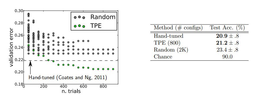
Hyperparameter tuning has traditionally been more art than science. If the number of hyperparameters is small, then you might be able to do a brute-force grid search to identify the hyperparameters that yield optimal model performance. As the number of hyperparameters increases, AI model builders often resort to random search through hyperparameter space.
However, there are also more structured approaches to hyperparameter optimization as described here.
Step 7: Model Deployment & Maintenance
Building machine learning models is more than just an academic exercise. It should be something that drives business value, and it can only do that once it is deployed.
Model deployment
You can deploy models directly on cloud servers such as AWS, Azure, or GCP. However, doing so necessitates setting up and maintaining an entire environment. Alternatively, you can use a platform like Viso to deploy your model with significantly less headache.
There are many platforms available to help make model deployment easier.
Model monitoring & maintenance
Once our model is deployed, we need to make sure nothing breaks it. If we’re running on AWS, Azure, or GCP, that means keeping libraries and containers updated. It may also mean establishing a CI/CD pipeline to automate model updates in the future. Ultimately, having a usable model in production is the end goal of our machine learning project.
Future Advancements
Machine learning is a rapidly changing field, and advancements are made daily and weekly, not yearly. Some of the current areas of cutting-edge research include:
- Multi-media transformer models,
- Human explainable AI,
- Machine learning models for quantum computers,
- Neural Radiance Fields (NeRFs),
- Privacy-preserving ML models using techniques like differential privacy and homomorphic encryption,
- Using synthetic data as part of the model training process, and
- Automating machine learning workflows using self-improving generative models.
Additionally, a significant amount of current research is dedicated to the development of AI “agents”. AI agents are essentially multi-step reasoning models that can iteratively define and then solve complex problems. Typically, AI agents can also directly perform actions such as searching the internet, sending an email, or submitting a form.
