


GoogLeNet, released in 2014, set a new benchmark in object classification and detection through its innovative approach (achieving a top-5 error rate of 6.7%, nearly half the error rate of the previous year’s winner ZFNet with 11.7%) in ImageNet Large Scale Visual Recognition Challenge (ILSVRC).
GoogLeNet’s deep learning model was deeper than all the previous models released, with 22 layers in total. Increasing the depth of the Machine Learning model is intuitive, as deeper models tend to have more learning capacity and as a result, this increases the performance of a model. However, this is only possible if we can solve the vanishing gradient problem.
When designing a deep learning model, one needs to decide what convolution filter size to use (whether it should be 3×3, 5×5, or 1×3) as it affects the model’s learning and performance, and when to max pool the layers. However, the inception module, the key innovation introduced by a team of Google researchers solved this problem creatively. Instead of deciding what filter size to use and when max pooling operation must be performed, they combined multiple convolution filters.
Stacking multiple convolution filters together instead of just one increases the parameter count many times. However, GoogLeNet demonstrated by using the inception module that depth and width in a neural network could be increased without exploding computations. We will investigate the inception module in depth.
Historical Context
The concept of Convolutional Neural Networks (CNNs) isn’t new. It dates back to the 1980s with the introduction of the Noncognition by Kunihiko Fukushima. However, CNNs gained popularity in the 1990s after Yann LeCun and his colleagues introduced LeNet-5 (one of the earliest CNNs), designed for handwritten digit recognition. LeNet-5 laid the groundwork for modern CNNs by using a series of convolutional layers followed by subsampling layers, now commonly referred to as pooling layers.
However, CNNs never saw any widespread adoption for a long time after LeNet-5, due to a lack of computational resources and the unavailability of large datasets, which made the learned models impotent.
The turning point came in 2012 with the introduction of AlexNet by Alex Krizhevsky, Ilya Sutskever, and Geoffrey Hinton. AlexNet was designed for the ImageNet challenge and significantly outperformed other machine learning approaches. This brought deep learning to the forefront of AI research. AlexNet featured several innovations, such as ReLU, dropout for regularization, and overlapping pooling.
After AlexNet, researchers started developing complex and deeper networks. GoogLeNet had 22 layers and VGGNet had 16 layers compared to AlexNet which had only 8 layers in total.
However, in the VGGNet paper, the limitations of simply stacking more layers were highlighted, as it was computationally expensive and led to overfitting. It wasn’t possible to keep increasing the layers without any innovation to cater to these problems.
Architecture of GoogLeNet
| type | patch size/stride | output size | depth | #1×1 | #3×3 reduce | #3×3 | #5×5 reduce | #5×5 | pool proj | params | ops |
|---|---|---|---|---|---|---|---|---|---|---|---|
| convolution | 7×7/2 | 112×112×64 | 1 | 2.7K | 34M | ||||||
| max pool | 3×3/2 | 56×56×64 | 0 | ||||||||
| convolution | 3×3/1 | 56×56×192 | 2 | 64 | 192 | 112K | 360M | ||||
| max pool | 3×3/2 | 28×28×192 | 0 | ||||||||
| inception (3a) | 28×28×256 | 2 | 64 | 96 | 128 | 16 | 32 | 32 | 159K | 128M | |
| inception (3b) | 28×28×480 | 2 | 128 | 128 | 192 | 32 | 96 | 64 | 380K | 304M | |
| max pool | 3×3/2 | 14×14×480 | 0 | ||||||||
| inception (4a) | 14×14×512 | 2 | 192 | 96 | 208 | 16 | 48 | 64 | 364K | 73M | |
| inception (4b) | 14×14×512 | 2 | 160 | 112 | 224 | 24 | 64 | 64 | 437K | 88M | |
| inception (4c) | 14×14×512 | 2 | 128 | 128 | 256 | 24 | 64 | 64 | 463K | 100M | |
| inception (4d) | 14×14×528 | 2 | 112 | 144 | 288 | 32 | 64 | 64 | 580K | 119M | |
| inception (4e) | 14×14×832 | 2 | 256 | 160 | 320 | 32 | 128 | 128 | 840K | 170M | |
| max pool | 3×3/2 | 7×7×832 | 0 | ||||||||
| inception (5a) | 7×7×832 | 2 | 256 | 160 | 320 | 32 | 128 | 128 | 1072K | 54M | |
| inception (5b) | 7×7×1024 | 2 | 384 | 192 | 384 | 48 | 128 | 128 | 1388K | 71M | |
| avg pool | 7×7/1 | 1x1x1024 | 0 | ||||||||
| dropout (40%) | 1x1x1024 | 0 | |||||||||
| linear | 1x1x1000 | 1 | 1000K | 1M | |||||||
| softmax | 1x1x1000 | 0 |
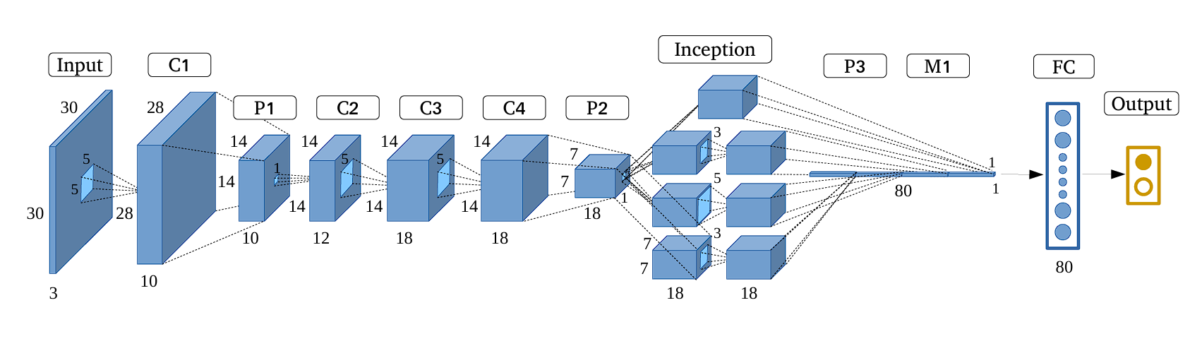
GoogLeNet model is particularly known for its use of Inception modules, which serve as its building blocks by using parallel convolutions with various filter sizes (1×1, 3×3, and 5×5) within a single layer. The outputs from these filters are then concatenated. This fusion of outputs from various filters creates a richer representation.
Moreover, the architecture is relatively deep with 22 layers, however, the model maintains computational efficiency despite the increase in the number of layers.
Here are the key features of GoogLeNet:
- Inception Module
- The 1×1 Convolution
- Global Average Pooling
- Auxiliary Classifiers for Training
The Inception Module
The Inception Module is the building block of GoogLeNet, as the entire model is made by stacking Inception Modules. Here are the key features of it:
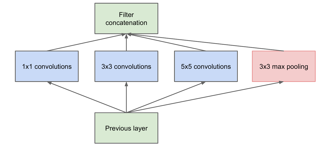
- Multi-Level Feature Extraction: The main idea of the inception module is that it consists of multiple pooling and convolution operations with different sizes (3×3, 5×5) in parallel, instead of using just one filter of a single size.
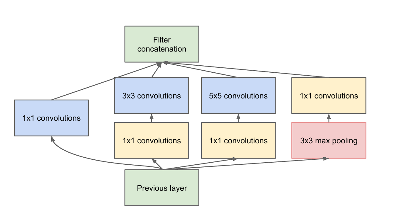
- Dimension Reduction: However, as we discussed earlier, stacking multiple layers of convolution results in increased computations. To overcome this, the researchers incorporate 1×1 convolution before feeding the data into 3×3 or 5×5 convolutions. This is also called dimensionality reduction.
To put it into perspective, let’s look at the difference.
- Input Feature Map Size: 28×28
- Input Channels (D): 192
- Number of Filters in 3×3 Convolution (F): 96
Without Reduction:
- Total Parameters=3×3×192×96=165,888
With Reduction:
- 1×1 Parameters=1×1×192×64=12,288
- 3×3 Parameters=3×3×64×96=55,296
- Total Parameters with Reduction=12,288+55,296=67,584
Benefits
- Parameter Efficiency: By using 1×1 convolutions, the module reduces dimensionality before applying the more expensive 3×3 and 5×5 convolutions and pooling operations.
- Increased Representation: By incorporating filters of varying sizes and more layers, the network captures a wide range of features in the input data. This results in better representation.
- Enhancing Feature Combination: The 1×1 convolution is also called network in the network. This means that each layer is a micro-neural network that learns to abstract the data before the main convolution filters are applied.
Global Average Pooling
Global Average Pooling is a technique used in Convolutional Neural Networks (CNNs) in the place of fully connected layers at the end part of the network. This method is used to reduce the total number of parameters and to minimize overfitting.
For example, consider you have a feature map with dimensions 10,10, 32 (Width, Height, Channels).
Global Average Pooling performs an average operation across the Width and Height for each filter channel separately. This reduces the feature map to a vector that is equal to the size of the number of channels.
The output vector captures the most prominent features by summarizing the activation of each channel across the entire feature map. Here our output vector is of the length 32, which is equal to the number of channels.
Benefits of Global Average Pooling
- Reduced Dimensionality: GAP significantly reduces the number of parameters in the network, making it efficient and faster during training and inference. Due to the absence of trainable parameters, the model is less prone to overfitting.
- Robustness to Spatial Variations: The entire feature map is summarized, as a result, GAP is less sensitive to small spatial shifts in the object’s location within the image.
- Computationally Efficient: It’s a simple operation compared to a set of fully connected layers.
In GoogLeNet architecture, replacing fully connected layers with global average pooling improved the top-1 accuracy by about 0.6%. In GoogLeNet, global average pooling can be found at the end of the network, where it summarizes the features learned by the CNN and then feeds it directly into the SoftMax classifier.
Auxiliary Classifiers for Training
These are intermediate classifiers found on the side of the network. One important thing to note is that these are only used during training and in the inference, these are omitted.
Auxiliary classifiers help overcome the challenges of training very Deep Neural Networks, and vanishing gradients (when the gradients turn into extremely small values).
In the GoogLeNet architecture, there are two auxiliary classifiers in the network. They are placed strategically, where the depth of the feature extracted is sufficient to make a meaningful impact, but before the final prediction from the output classifier.
The structure of each auxiliary classifier is mentioned below:
- An average pooling layer with a 5×5 window and stride 3.
- A 1×1 convolution for dimension reduction with 128 filters.
- Two fully connected layers, the first layer with 1024 units, followed by a dropout layer and the final layer corresponding to the number of classes in the task.
- A SoftMax layer to output the prediction probabilities.
During training, the loss calculated from each auxiliary classifier is weighted and added to the total loss of the network. In the original paper, it is set to 0.3.
These auxiliary classifiers help the gradient to flow and not diminish too quickly, as it propagates back through the deeper layers. This is what makes training a Deep Neural Network like GoogLeNet possible.
Moreover, the auxiliary classifiers also help with model regularization. Since each classifier contributes to the final output, as a result, the network is encouraged to distribute its learning across different parts of the network. This distribution prevents the network from relying too heavily on specific features or layers, which reduces the chances of overfitting.
Performance of GoogLeNet
GoogLeNet achieved a top-5 error rate of 6.67%, improving the score compared to previous models.
Here is a comparison with other models released previously:
| Team | Year | Place | Error (top-5) | Uses External Data |
|---|---|---|---|---|
| SuperVision | 2012 | 1st | 16.4% | no |
| SuperVision | 2012 | 1st | 15.3% | Imagenet 22k |
| Clarifai | 2013 | 1st | 11.7% | no |
| Clarifai | 2013 | 1st | 11.2% | Imagenet 22k |
| MSRA | 2014 | 3rd | 7.32% | no |
| VGG | 2014 | 2nd | 7.32% | no |
| GoogLeNet | 2014 | 1st | 6.67% | no |
Comparison with Other Architectures
- AlexNet (2012): Top-5 Error Rate of 15.3%. The Architecture Consists of 8 layers (5 convolutional and 3 fully connected layers), which used ReLU activations, dropout, and data augmentation to achieve state-of-the-art performance in 2012.
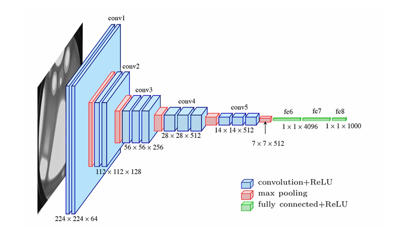
- VGG (2014): Top-5 Error Rate of 7.3%. The Architecture is appreciated for its simplicity, using only 3×3 convolutional layers stacked on top of each other in increasing depth. Moreover, VGG was also the runner-up in the same competition that GoogLeNet won. Although VGG used small convolution filters, its parameter count, and computation were intensive compared to GoogLeNet.
GoogLeNet Variants and Successors
Following the success of the original Google Net (Inception v1), several variants and successors were developed to enhance its architecture. These include Inception v2, v3, v4, and the Inception-ResNet hybrids. Each of these models introduced key improvements and optimizations. These addressed various challenges and pushed the boundaries of what was possible with the CNN architectures.
- Inception v2 (2015): The second version of Inception was modified with improvements such as batch normalization and shortcut connections. It also refined the inception modules by replacing larger convolutions with smaller, more efficient ones. These changes improved accuracy and reduced training time.
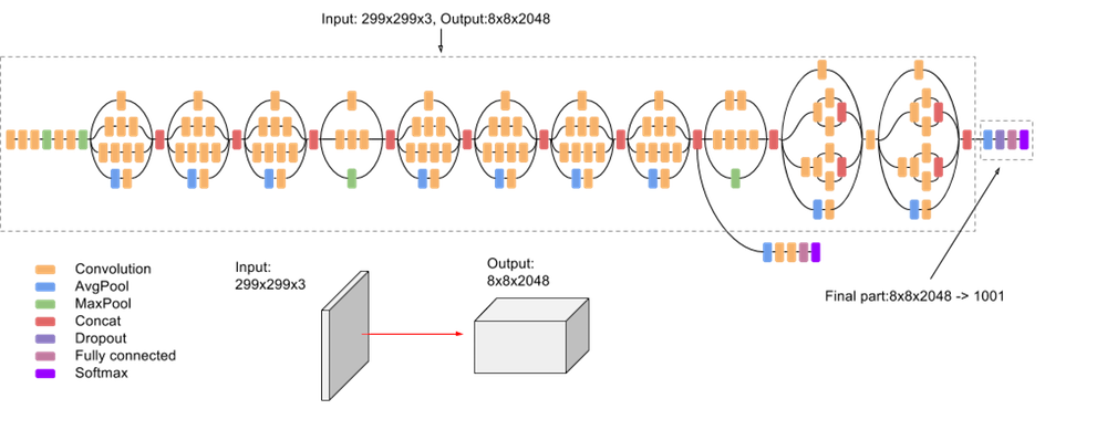
- Inception v3 (2015): The v3 model further refined Inception v2 by using atrous convolution (dilated convolutions that expand the network’s receptive field without sacrificing resolution and significantly increasing network parameters).
- Inception v4, Inception-ResNet v2 (2016): This version of Inception introduced residual connections (inspired by ResNet) into the Inception lineage, which led to further performance improvements.
- Xception (2017): Xception replaced Inception modules with depth-wise separable convolutions.
- MobileNet (2017): This architecture is for mobile and embedded devices. The network uses depth-wise separable convolutions and linear bottleneck layers.
- EfficientNet (2019): This is a family of models that scales both model size and accuracy strategically by using Neural Architecture Search (NAS).
Conclusion
GoogLeNet, or Inception v1, contributed significantly to the development of CNNs with the introduction of the inception module. Its use of diverse convolution filters in a single layer expanded the network and 1×1 convolutions for dimensionality reduction.
As a result of the innovations, it won the ImageNet challenge with a record-low error rate. However, it shows researchers how they can develop a deeper model without increasing computational demands significantly. As a result, its successors, like Inception v2, v3, etc., built on the core ideas to achieve even greater performance and flexibility.
To learn more about computer vision and machine learning, check out the other articles on the viso.ai blog:
- AI at the Edge: Using NVIDIA Jetson
- AI Hardware: Google Coral
- Open Source Computer Vision with OpenCV
- Deep Learning vs. Machine Learning: An In-Depth Comparison
- The Ultimate Guide to AI Models