Long Short-Term Memory (LSTM) is a structure that can be used in neural network. It is a type of recurrent neural network (RNN) that expects the input in the form of a sequence of features. It is useful for data such as time series or string of text. In this post, you will learn about LSTM networks. In particular,
What is LSTM and how they are different
How to develop LSTM network for time series prediction
How to train a LSTM network
Kick-start your project with my book Deep Learning with PyTorch. It provides self-study tutorials with working code.
Let’s get started.
LSTM for Time Series Prediction in PyTorch Photo by Carry Kung. Some rights reserved.
Overview
This post is divided into three parts; they are
Overview of LSTM Network
LSTM for Time Series Prediction
Training and Verifying Your LSTM Network
Overview of LSTM Network
LSTM cell is a building block that you can use to build a larger neural network. While the common building block such as fully-connected layer are merely matrix multiplication of the weight tensor and the input to produce an output tensor, LSTM module is much more complex.
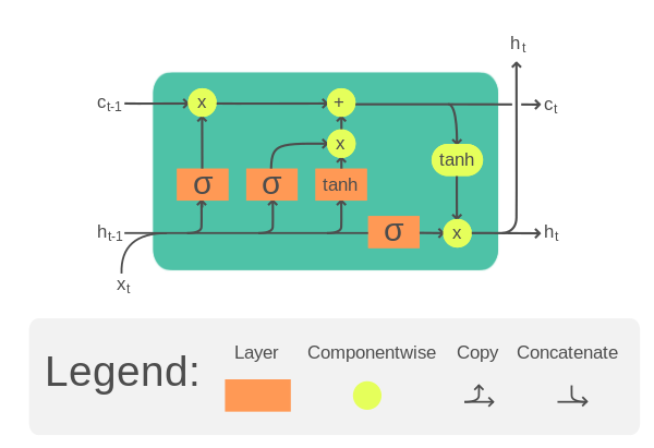
A typical LSTM cell is illustrated as follows
LSTM cell. Illustration from Wikipedia.
It takes one time step of an input tensor $x$ as well as a cell memory $c$ and a hidden state $h$. The cell memory and hidden state can be initialized to zero at the beginning. Then within the LSTM cell, $x$, $c$, and $h$ will be multiplied by separate weight tensors and pass through some activation functions a few times. The result is the updated cell memory and hidden state. These updated $c$ and $h$ will be used on the **next time step** of the input tensor. Until the end of the last time step, the output of the LSTM cell will be its cell memory and hidden state.
Specifically, the equation of one LSTM cell is as follows:
Where $W$, $U$, $b$ are trainable parameters of the LSTM cell. Each equation above is computed for each time step, hence with subscript $t$. These trainable parameters are reused for all the time steps. This nature of shared parameter bring the memory power to the LSTM.
Note that the above is only one design of the LSTM. There are multiple variations in the literature.
Since the LSTM cell expects the input $x$ in the form of multiple time steps, each input sample should be a 2D tensors: One dimension for time and another dimension for features. The power of an LSTM cell depends on the size of the hidden state or cell memory, which usually has a larger dimension than the number of features in the input.
Want to Get Started With Deep Learning with PyTorch?
Take my free email crash course now (with sample code).
Click to sign-up and also get a free PDF Ebook version of the course.
LSTM for Time Series Prediction
Let’s see how LSTM can be used to build a time series prediction neural network with an example.
The problem you will look at in this post is the international airline passengers prediction problem. This is a problem where, given a year and a month, the task is to predict the number of international airline passengers in units of 1,000. The data ranges from January 1949 to December 1960, or 12 years, with 144 observations.
It is a regression problem. That is, given the number of passengers (in unit of 1,000) the recent months, what is the number of passengers the next month. The dataset has only one feature: The number of passengers.
Let’s start by reading the data. The data can be downloaded here.
Save this file as airline-passengers.csv in the local directory for the following.
Below is a sample of the first few lines of the file:
1
2
3
4
5
"Month","Passengers"
"1949-01",112
"1949-02",118
"1949-03",132
"1949-04",129
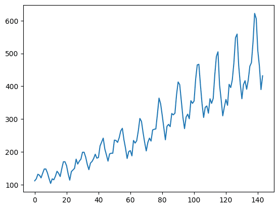
The data has two columns, the month and the number of passengers. Since the data are arranged in chronological order, you can take only the number of passenger to make a single-feature time series. Below you will use pandas library to read the CSV file and convert it into a 2D numpy array, then plot it using matplotlib:
This time series has 144 time steps. You can see from the plot that there is an upward trend. There are also some periodicity in the dataset that corresponds to the summer holiday period in the northern hemisphere. Usually a time series should be “detrended” to remove the linear trend component and normalized before processing. For simplicity, these are skipped in this project.
To demonstrate the predictive power of our model, the time series is splitted into training and test sets. Unlike other dataset, usually time series data are splitted without shuffling. That is, the training set is the first half of time series and the remaining will be used as the test set. This can be easily done on a numpy array:
The more complicated problem is how do you want the network to predict the time series. Usually time series prediction is done on a window. That is, given data from time $t-w$ to time $t$, you are asked to predict for time $t+1$ (or deeper into the future). The size of window $w$ governs how much data you are allowed to look at when you make the prediction. This is also called the look back period.
On a long enough time series, multiple overlapping window can be created. It is convenient to create a function to generate a dataset of fixed window from a time series. Since the data is going to be used in a PyTorch model, the output dataset should be in PyTorch tensors:
1
2
3
4
5
6
7
8
9
10
11
12
13
14
15
16
import torch
def create_dataset(dataset,lookback):
"""Transform a time series into a prediction dataset
Args:
dataset: A numpy array of time series, first dimension is the time steps
lookback: Size of window for prediction
"""
X,y=[],[]
foriinrange(len(dataset)-lookback):
feature=dataset[i:i+lookback]
target=dataset[i+1:i+lookback+1]
X.append(feature)
y.append(target)
returntorch.tensor(X),torch.tensor(y)
This function is designed to apply windows on the time series. It is assumed to predict for one time step into the immediate future. It is designed to convert a time series into a tensor of dimensions (window sample, time steps, features). A time series of $L$ time steps can produce roughly $L$ windows (because a window can start from any time step as long as the window does not go beyond the boundary of the time series). Within one window, there are multiple consecutive time steps of values. In each time step, there can be multiple features. In this dataset, there is only one.
It is intentional to produce the “feature” and the “target” the same shape: For a window of three time steps, the “feature” is the time series from $t$ to $t+2$ and the target is from $t+1$ to $t+3$. What we are interested is $t+3$ but the information of $t+1$ to $t+2$ is useful in training.
Note that the input time series is a 2D array and the output from the create_dataset() function will be a 3D tensors. Let’s try with lookback=1. You can verify the shape of the output tensor as follows:
Now you can build the LSTM model to predict the time series. With lookback=1, it is quite surely that the accuracy would not be good for too little clues to predict. But this is a good example to demonstrate the structure of the LSTM model.
The model is created as a class, in which a LSTM layer and a fully-connected layer is used.
The output of nn.LSTM() is a tuple. The first element is the generated hidden states, one for each time step of the input. The second element is the LSTM cell’s memory and hidden states, which is not used here.
The LSTM layer is created with option batch_first=True because the tensors you prepared is in the dimension of (window sample, time steps, features) and where a batch is created by sampling on the first dimension.
The output of hidden states is further processed by a fully-connected layer to produce a single regression result. Since the output from LSTM is one per each input time step, you can chooce to pick only the last timestep’s output, which you should have:
1
2
3
4
x,_=self.lstm(x)
# extract only the last time step
x=x[:,-1,:]
x=self.linear(x)
and the model’s output will be the prediction of the next time step. But here, the fully connected layer is applied to each time step. In this design, you should extract only the last time step from the model output as your prediction. However, in this case, the window is 1, there is no difference in these two approach.
Training and Verifying Your LSTM Network
Because it is a regression problem, MSE is chosen as the loss function, which is to be minimized by Adam optimizer. In the code below, the PyTorch tensors are combined into a dataset using torch.utils.data.TensorDataset() and batch for training is provided by a DataLoader. The model performance is evaluated once per 100 epochs, on both the trainning set and the test set:
print("Epoch %d: train RMSE %.4f, test RMSE %.4f"%(epoch,train_rmse,test_rmse))
As the dataset is small, the model should be trained for long enough to learn about the pattern. Over these 2000 epochs trained, you should see the RMSE on both training set and test set decreasing:
1
2
3
4
5
6
7
8
9
10
11
12
13
14
15
16
17
18
19
20
Epoch 0: train RMSE 225.7571, test RMSE 422.1521
Epoch 100: train RMSE 186.7353, test RMSE 381.3285
Epoch 200: train RMSE 153.3157, test RMSE 345.3290
Epoch 300: train RMSE 124.7137, test RMSE 312.8820
Epoch 400: train RMSE 101.3789, test RMSE 283.7040
Epoch 500: train RMSE 83.0900, test RMSE 257.5325
Epoch 600: train RMSE 66.6143, test RMSE 232.3288
Epoch 700: train RMSE 53.8428, test RMSE 209.1579
Epoch 800: train RMSE 44.4156, test RMSE 188.3802
Epoch 900: train RMSE 37.1839, test RMSE 170.3186
Epoch 1000: train RMSE 32.0921, test RMSE 154.4092
Epoch 1100: train RMSE 29.0402, test RMSE 141.6920
Epoch 1200: train RMSE 26.9721, test RMSE 131.0108
Epoch 1300: train RMSE 25.7398, test RMSE 123.2518
Epoch 1400: train RMSE 24.8011, test RMSE 116.7029
Epoch 1500: train RMSE 24.7705, test RMSE 112.1551
Epoch 1600: train RMSE 24.4654, test RMSE 108.1879
Epoch 1700: train RMSE 25.1378, test RMSE 105.8224
Epoch 1800: train RMSE 24.1940, test RMSE 101.4219
Epoch 1900: train RMSE 23.4605, test RMSE 100.1780
It is expected to see the RMSE of test set is an order of magnitude larger. The RMSE of 100 means the prediction and the actual target would be in average off by 100 in value (i.e., 100,000 passengers in this dataset).
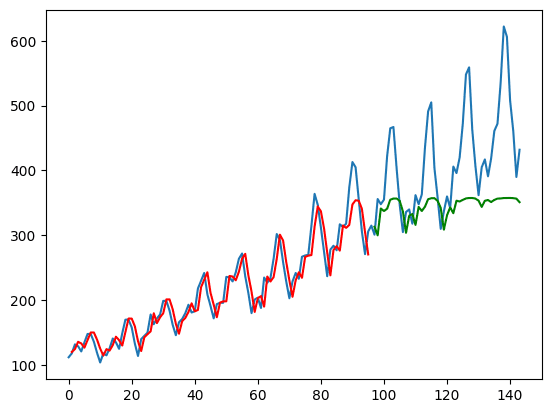
To better understand the prediction quality, you can indeed plot the output using matplotlib, as follows:
From the above, you take the model’s output as y_pred but extract only the data from the last time step as y_pred[:, -1, :]. This is what is plotted on the chart.
The training set is plotted in red while the test set is plotted in green. The blue curve is what the actual data looks like. You can see that the model can fit well to the training set but not very well on the test set.
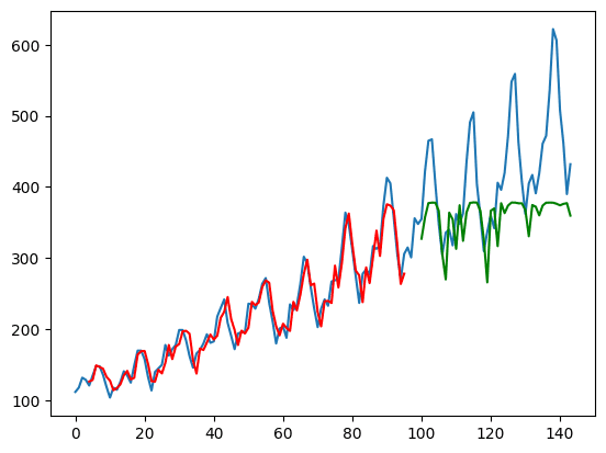
Tying together, below is the complete code, except the parameter lookback is set to 4 this time:
Running the above code will produce the plot below. From both the RMSE measure printed and the plot, you can notice that the model can now do better on the test set.
This is also why the create_dataset() function is designed in such way: When the model is given a time series of time $t$ to $t+3$ (as lookback=4), its output is the prediction of $t+1$ to $t+4$. However, $t+1$ to $t+3$ are also known from the input. By using these in the loss function, the model effectively was provided with more clues to train. This design is not always suitable but you can see it is helpful in this particular example.
Further Readings
This section provides more resources on the topic if you are looking to go deeper.
It provides self-study tutorials with hundreds of working code to turn you from a novice to expert. It equips you with tensor operation, training, evaluation, hyperparameter optimization,
and much more...
Kick-start your deep learning journey with hands-on exercises
Forgive me, there must be an error somewhere:
print(X_train.shape, y_train.shape)
print(X_test.shape, y_test.shape)
torch.Size([95, 1]) torch.Size([95, 1])
torch.Size([47, 1]) torch.Size([47, 1])
Hi James, I apologize I wrote the comment too hastily, the error was mine, the shape of my timeseries was (432,) while yours is (432,1) this generated in the create_dataset(dataset, lookback) function an incorrect tensor shape: torch.Size([95, 1]) torch.Size([95, 1]) torch.Size([47, 1]) torch.Size([47, 1]) and not the correct one: torch.Size([95, 1, 1]) torch.Size([95, 1, 1]) torch.Size([47, 1, 1]) torch.Size([47, 1, 1]) as in your example.
I just added X=np.array(X) and y np.array(y) before return torch.tensor(X), torch.tensor(y) to avoid the message “UserWarning: Creating a tensor from a list of numpy.ndarrays is extremely slow…”. Thank you for sharing your excellent work.
Hi James, I’m wondering, if we use the “create_dataset” function to create the windows for the training, after training the model and using it ti predict we will need to transform our new dataset and have the same shape to predict, therefore, we won’t predict for the last “N lookback” instances due to the function is only getting windows for “len(dataset)-lookback”. In conclusion, we won’t predict values for the whole dataset, if I use lookback=3, I won’t get predictions for the last 3 instances.
Hi Sobiedd…I am not certain I am following your question. Have you performed a prediction and have noted an issue with the suggested methodology used in the tutorial? Perhaps we can start with your results and determine if there is something missing from the implementation.
Hi Jason! Thanks for this blog, it’s really helpful. I intended to use the lstm network for prediction. The dataset I have is a social media dataset with multiple variables(image features, posts posting date, tags, location info etc.). This dataset has temporal features, so I can plot each post v/s the output, taking month-year(the time scale) on x-axis and o/p on y-axis.
I have done the feature engineering and now I wanted to train a lstm model to predict the output. But since NN/lstm models need data to be normalized, I was wondering –
1.) whether to normalize/scale the data,
2.) should I normalize considering each feature for each samples? or should I normalize it feature-wise(normalize by tags_length feature/column)?
I need your suggestion as early as possible since I’m aiming for a deadline. Any help is highly appreciated. I look forward to your suggestion. Thank You!
Perhaps I am wrong, but it seems that you are using teacher forcing during the test phase. It doesn’t seem like the model is autoregressive. I would like to see results where the LSTM uses its own predictions to generate new ones.
If I have to predict several consecutive future time-series values, how can I do it? For example, if I have predictor variables and target till now (t=0), how can I predict the target at t+1, t+2, and t+3? In other words, if I have the predictor variables and target for every hour (as historical data), how can I predict the values of the target for the upcoming three hours? How can I prepare the dataset and update my model (e.g., LSTM)?
The samples may be shuffled because each sample is independent. That is, a given sample captures an entire input sequence; therefore, sequential information is retained even as samples are shuffled.
You are working on a time series forecasting problem and you plot your forecasted time series against the actual time series and it looks like the forecast is one step behind the actual.
This is common.
It means that your model is making a persistence forecast. This is a forecast where the input to the forecast (e.g. the observation at the previous time step) is predicted as the output.
The persistence forecast is used as a baseline method for comparison on time series forecasting. You can learn more about the method here:
How to Make Baseline Predictions for Time Series Forecasting with Python
The persistence forecast is the best that we can do on challenging time series forecasting problems, such as those series that are a random walk, like short range movements of stock prices. You can learn more about this here:
A Gentle Introduction to the Random Walk for Times Series Forecasting with Python
If your sophisticated model, such as a neural network, is outputting a persistence forecast, it might mean:
That the model requires further tuning.
That the chosen model cannot address your specific dataset.
It might also mean that your time series problem is not predictable.
Hi there,
All those tutorials refer to forecast training and testing, but can you do a one which actually forecast beyond the dataset as example next 3 .months forecast
Looking at your final graph above, it appears that the trained model is still only doing a persistence forecast as it is almost an exact shifted version of the dataset. Is that a reflection of an issue in this lookback approach implementation in general or is it a reflection of the lack of useful features in the dataset? How would you proceed from here to make it more accurate?
Hi Michael…You are working on a time series forecasting problem and you plot your forecasted time series against the actual time series and it looks like the forecast is one step behind the actual.
This is common.
It means that your model is making a persistence forecast. This is a forecast where the input to the forecast (e.g. the observation at the previous time step) is predicted as the output.
The persistence forecast is used as a baseline method for comparison on time series forecasting. You can learn more about the method here:
How to Make Baseline Predictions for Time Series Forecasting with Python
The persistence forecast is the best that we can do on challenging time series forecasting problems, such as those series that are a random walk, like short range movements of stock prices. You can learn more about this here:
A Gentle Introduction to the Random Walk for Times Series Forecasting with Python
If your sophisticated model, such as a neural network, is outputting a persistence forecast, it might mean:
That the model requires further tuning.
That the chosen model cannot address your specific dataset.
It might also mean that your time series problem is not predictable.
I played a bit with your code and I note that if I adjust the settings to eliminate the persistence shift on the trained set by increasing lookback or network size, I end up over fitting and getting even worse performance on the test set, so I get the impression this is a hard tradeoff in the case of this lookback lstm stackup. I read the other material, it is helpful, but doesn’t show me a way out of this tradeoff of either overfitting or persistence.
1 – Is ‘hidden_size’ from Pytorch the same parameter as ‘units’ in Tensorflow/Keras?
2 – If yes, what they actually represent in the first figure in this post? For example, if we have ‘hidden_size = X’, we have X LSTM cells? Or when we define ‘nn.LSTM(input_size=1, hidden_size=X, num_layers=1, batch_first=True)’ we have one cell no matter the value of X?
3 – And how they are conected to the linear/dense layer? Each cell is conected to each node in the linear layer? Or just the last cell is conected to each node?
Hi. I have a question to confirm my observation. Does the number of records on both training and test splits lessened based on the number of lookbacks? For instance in my case, there were 699 records for the original train split which became 698 after applying create_dataset() function. The same happened for my test wherein from 48, it became 47.
The same length was also applied for train and test predictions. I also have another question with regards to displaying the plot. Since the number of train and test predictions are different from the number of records from the original train and test splits, how should I plot it with the x-axis as the datetime stamp?
Hi J…Based on your description, it sounds like you are observing a common behavior in time series data preparation when using a function like create_dataset() which typically is used to reformat a time series dataset into a format suitable for LSTM models, by creating lookback sequences. Let’s clarify and answer both parts of your question:
### Reduction in Records Due to Lookbacks
The reduction in the number of records from your original dataset to what you have after applying the create_dataset() function is indeed expected due to the nature of lookback processing. Here’s how it works:
– **Lookback Logic**: If you are using a lookback period (also known as lag, window size, or sequence length), the function needs to create sequences of that many past observations to predict the current value. For example, with a lookback of 1, each input sequence for your model will consist of one previous time step to predict the current time step.
– **Effect on Data Size**: This means that the first few records in your dataset (exactly as many as your lookback period) won’t have enough previous data points to form a complete sequence. Thus, these records are typically dropped from the training or testing datasets. For a lookback of 1, you lose 1 data point at the start, which matches what you observed: 699 records becoming 698, and 48 becoming 47.
### Plotting Data with Mismatched Lengths
Regarding plotting the training and test predictions alongside the original data with timestamps on the x-axis, considering the mismatch in lengths due to the lookback, you can handle this by adjusting the index of your predictions. Here’s how you can do it:
1. **Offset Adjustments**: Since each prediction corresponds to an output where the input sequence ends, you should start plotting predictions from the index equivalent to the lookback period. For example, if your lookback is 1, your predictions should start from the second record in your original dataset.
2. **Code Example**: Suppose your DataFrame with the original time series is df, and it includes a datetime column date. Here’s a basic plotting approach using Python and matplotlib:
python

import matplotlib.pyplot as plt
# Sample data
dates = df['date'] # Assuming 'date' is your datetime column
original_train = df['value'][:698] # Assuming 'value' is what you're predicting
original_test = df['value'][698:]
# Assuming train_predictions and test_predictions are your model outputs
train_predictions = [None] + list(train_predictions) # Offset for alignment
test_predictions = [None] * 699 + list(test_predictions) # Offset for alignment
– **Alignment by Index**: The None values are added to the predictions list to align the predictions correctly with the original data indices. Adjust the number of None values based on your exact lookback and how your splits are structured.
– **Plotting All Together**: This script plots the original data along with the adjusted predictions on the same graph for visual comparison.
This approach will help you visually compare how well your model’s predictions match up against the actual values, taking into account the datetime sequence. Adjust the plotting details as needed to fit your specific setup and visualization needs.


Forgive me, there must be an error somewhere:
print(X_train.shape, y_train.shape)
print(X_test.shape, y_test.shape)
torch.Size([95, 1]) torch.Size([95, 1])
torch.Size([47, 1]) torch.Size([47, 1])
Hi Eliasnemo…What is the error you are referring to?
Hi James, I apologize I wrote the comment too hastily, the error was mine, the shape of my timeseries was (432,) while yours is (432,1) this generated in the create_dataset(dataset, lookback) function an incorrect tensor shape: torch.Size([95, 1]) torch.Size([95, 1]) torch.Size([47, 1]) torch.Size([47, 1]) and not the correct one: torch.Size([95, 1, 1]) torch.Size([95, 1, 1]) torch.Size([47, 1, 1]) torch.Size([47, 1, 1]) as in your example.
I just added X=np.array(X) and y np.array(y) before return torch.tensor(X), torch.tensor(y) to avoid the message “UserWarning: Creating a tensor from a list of numpy.ndarrays is extremely slow…”. Thank you for sharing your excellent work.
Hi, this post is informative! In line 65-68, should it be X_batch and y_batch instead of X_train and y_train?
Hi tqrahman…I do not see an error. What is your results by changing the code to that for which you suggested?
do you have example for predict next x day graph plot
Hi guest…please clarify your question so that we may better assist you.
Hi James, I’m wondering, if we use the “create_dataset” function to create the windows for the training, after training the model and using it ti predict we will need to transform our new dataset and have the same shape to predict, therefore, we won’t predict for the last “N lookback” instances due to the function is only getting windows for “len(dataset)-lookback”. In conclusion, we won’t predict values for the whole dataset, if I use lookback=3, I won’t get predictions for the last 3 instances.
Hi Sobiedd…I am not certain I am following your question. Have you performed a prediction and have noted an issue with the suggested methodology used in the tutorial? Perhaps we can start with your results and determine if there is something missing from the implementation.
Hi Jason! Thanks for this blog, it’s really helpful. I intended to use the lstm network for prediction. The dataset I have is a social media dataset with multiple variables(image features, posts posting date, tags, location info etc.). This dataset has temporal features, so I can plot each post v/s the output, taking month-year(the time scale) on x-axis and o/p on y-axis.
I have done the feature engineering and now I wanted to train a lstm model to predict the output. But since NN/lstm models need data to be normalized, I was wondering –
1.) whether to normalize/scale the data,
2.) should I normalize considering each feature for each samples? or should I normalize it feature-wise(normalize by tags_length feature/column)?
I need your suggestion as early as possible since I’m aiming for a deadline. Any help is highly appreciated. I look forward to your suggestion. Thank You!
Hi James,
Perhaps I am wrong, but it seems that you are using teacher forcing during the test phase. It doesn’t seem like the model is autoregressive. I would like to see results where the LSTM uses its own predictions to generate new ones.
Hi Angelo…The following example may help add clarity:
https://machinelearningmastery.com/how-to-develop-lstm-models-for-multi-step-time-series-forecasting-of-household-power-consumption/
Hi James,
If I have to predict several consecutive future time-series values, how can I do it? For example, if I have predictor variables and target till now (t=0), how can I predict the target at t+1, t+2, and t+3? In other words, if I have the predictor variables and target for every hour (as historical data), how can I predict the values of the target for the upcoming three hours? How can I prepare the dataset and update my model (e.g., LSTM)?
Thank you.
Hi James,
I’m just checking – in the snipper where you extract the last step, are we missing a colon after the “-1”?
Something like
x = x[:, -1:, :]
Hi Tom…Thank you for your feedback! We do not see an issue with the original code. What did you find when you executed it?
Given time series nature of the input, why did you set shuffle=true in DataLoader?
Hi Myk…The following resource may be of interest:
https://machinelearningmastery.com/training-a-pytorch-model-with-dataloader-and-dataset/#:~:text=The%20batch%20size%20is%20a,to%20read%20every%20batch%20once.
The samples may be shuffled because each sample is independent. That is, a given sample captures an entire input sequence; therefore, sequential information is retained even as samples are shuffled.
In your “complete code” above, lines 74-75 are redundant, as line 76 does the same thing:
y_pred = model(X_train)
y_pred = y_pred[:, -1, :]
train_plot[lookback:train_size] = model(X_train)[:, -1, :]
Both graphs seem to be shifted in both train and test plot. Why is that happening? And how to fix it?
You are working on a time series forecasting problem and you plot your forecasted time series against the actual time series and it looks like the forecast is one step behind the actual.
This is common.
It means that your model is making a persistence forecast. This is a forecast where the input to the forecast (e.g. the observation at the previous time step) is predicted as the output.
The persistence forecast is used as a baseline method for comparison on time series forecasting. You can learn more about the method here:
How to Make Baseline Predictions for Time Series Forecasting with Python
The persistence forecast is the best that we can do on challenging time series forecasting problems, such as those series that are a random walk, like short range movements of stock prices. You can learn more about this here:
A Gentle Introduction to the Random Walk for Times Series Forecasting with Python
If your sophisticated model, such as a neural network, is outputting a persistence forecast, it might mean:
That the model requires further tuning.
That the chosen model cannot address your specific dataset.
It might also mean that your time series problem is not predictable.
Hi there,
All those tutorials refer to forecast training and testing, but can you do a one which actually forecast beyond the dataset as example next 3 .months forecast
Hi Saranga…The following resource may be of interest to you:
https://stackoverflow.com/questions/69906416/forecast-future-values-with-lstm-in-python
Does LSTM works for time series classification?
Looking at your final graph above, it appears that the trained model is still only doing a persistence forecast as it is almost an exact shifted version of the dataset. Is that a reflection of an issue in this lookback approach implementation in general or is it a reflection of the lack of useful features in the dataset? How would you proceed from here to make it more accurate?
Hi Michael…You are working on a time series forecasting problem and you plot your forecasted time series against the actual time series and it looks like the forecast is one step behind the actual.
This is common.
It means that your model is making a persistence forecast. This is a forecast where the input to the forecast (e.g. the observation at the previous time step) is predicted as the output.
The persistence forecast is used as a baseline method for comparison on time series forecasting. You can learn more about the method here:
How to Make Baseline Predictions for Time Series Forecasting with Python
The persistence forecast is the best that we can do on challenging time series forecasting problems, such as those series that are a random walk, like short range movements of stock prices. You can learn more about this here:
A Gentle Introduction to the Random Walk for Times Series Forecasting with Python
If your sophisticated model, such as a neural network, is outputting a persistence forecast, it might mean:
That the model requires further tuning.
That the chosen model cannot address your specific dataset.
It might also mean that your time series problem is not predictable.
I played a bit with your code and I note that if I adjust the settings to eliminate the persistence shift on the trained set by increasing lookback or network size, I end up over fitting and getting even worse performance on the test set, so I get the impression this is a hard tradeoff in the case of this lookback lstm stackup. I read the other material, it is helpful, but doesn’t show me a way out of this tradeoff of either overfitting or persistence.
I have a few questions:
1 – Is ‘hidden_size’ from Pytorch the same parameter as ‘units’ in Tensorflow/Keras?
2 – If yes, what they actually represent in the first figure in this post? For example, if we have ‘hidden_size = X’, we have X LSTM cells? Or when we define ‘nn.LSTM(input_size=1, hidden_size=X, num_layers=1, batch_first=True)’ we have one cell no matter the value of X?
3 – And how they are conected to the linear/dense layer? Each cell is conected to each node in the linear layer? Or just the last cell is conected to each node?
Is the next line correct ?
target = dataset[i+1:i+lookback+1]
Because we want as target the next direct output, it should be:
target = dataset[i+lookback:i+lookback+1]
Hi Alexander…It should be correct. Did you execute the code? If so what did you find?
Hi. I have a question to confirm my observation. Does the number of records on both training and test splits lessened based on the number of lookbacks? For instance in my case, there were 699 records for the original train split which became 698 after applying create_dataset() function. The same happened for my test wherein from 48, it became 47.
The same length was also applied for train and test predictions. I also have another question with regards to displaying the plot. Since the number of train and test predictions are different from the number of records from the original train and test splits, how should I plot it with the x-axis as the datetime stamp?
Hi J…Based on your description, it sounds like you are observing a common behavior in time series data preparation when using a function like
create_dataset()which typically is used to reformat a time series dataset into a format suitable for LSTM models, by creating lookback sequences. Let’s clarify and answer both parts of your question:### Reduction in Records Due to Lookbacks
The reduction in the number of records from your original dataset to what you have after applying the
create_dataset()function is indeed expected due to the nature of lookback processing. Here’s how it works:– **Lookback Logic**: If you are using a lookback period (also known as lag, window size, or sequence length), the function needs to create sequences of that many past observations to predict the current value. For example, with a lookback of 1, each input sequence for your model will consist of one previous time step to predict the current time step.
– **Effect on Data Size**: This means that the first few records in your dataset (exactly as many as your lookback period) won’t have enough previous data points to form a complete sequence. Thus, these records are typically dropped from the training or testing datasets. For a lookback of 1, you lose 1 data point at the start, which matches what you observed: 699 records becoming 698, and 48 becoming 47.
### Plotting Data with Mismatched Lengths
Regarding plotting the training and test predictions alongside the original data with timestamps on the x-axis, considering the mismatch in lengths due to the lookback, you can handle this by adjusting the index of your predictions. Here’s how you can do it:
1. **Offset Adjustments**: Since each prediction corresponds to an output where the input sequence ends, you should start plotting predictions from the index equivalent to the lookback period. For example, if your lookback is 1, your predictions should start from the second record in your original dataset.
2. **Code Example**: Suppose your DataFrame with the original time series is
df, and it includes a datetime columndate. Here’s a basic plotting approach using Python and matplotlib:pythonimport matplotlib.pyplot as plt
# Sample data
dates = df['date'] # Assuming 'date' is your datetime column
original_train = df['value'][:698] # Assuming 'value' is what you're predicting
original_test = df['value'][698:]
# Assuming train_predictions
andtest_predictionsare your model outputstrain_predictions = [None] + list(train_predictions) # Offset for alignment
test_predictions = [None] * 699 + list(test_predictions) # Offset for alignment
plt.figure(figsize=(15, 8))
plt.plot(dates, df['value'], label='Original Data')
plt.plot(dates, train_predictions, label='Train Predictions')
plt.plot(dates, test_predictions, label='Test Predictions')
plt.legend()
plt.title('Time Series Prediction')
plt.xlabel('Date')
plt.ylabel('Value')
plt.show()
**Key Points in the Plotting Code:**
– **Alignment by Index**: The
Nonevalues are added to the predictions list to align the predictions correctly with the original data indices. Adjust the number ofNonevalues based on your exact lookback and how your splits are structured.– **Plotting All Together**: This script plots the original data along with the adjusted predictions on the same graph for visual comparison.
This approach will help you visually compare how well your model’s predictions match up against the actual values, taking into account the datetime sequence. Adjust the plotting details as needed to fit your specific setup and visualization needs.
If we add a single line logging the time series in the first cell:
timeseries = np.log(timeseries)
We get an almost perfect fit against the test set.
Hi Half Dome…Thank you for your feedback and suggestion!