Anomaly detection using Isolation Forest – A Complete Guide

Introduction

Anomaly detection is crucial in data mining and machine learning, finding applications in fraud detection, network security, and more. The Isolation Forest algorithm, introduced by Fei Tony Liu and Zhi-Hua Zhou in 2008, stands out among anomaly detection methods. It uses decision trees to efficiently isolate anomalies by randomly selecting features and splitting data based on threshold values. This approach is effective in quickly identifying outliers, making it well-suited for large datasets where anomalies are rare and distinct.

In this article, we delve into the workings of the Isolation Forest algorithm, its implementation in Python, and its role as a powerful tool in anomaly detection. We also explore the metrics used to evaluate its performance and discuss its applications across various domains.

Learning Outcomes

• Understand the concept of Average Path Length (APL) in the context of decision trees and its relevance in anomaly detection.
• Explain the structure and functionality of Binary Search Trees (BSTs) and their application in organizing data for efficient search operations.
• Apply data analysis techniques to analyze and interpret data stored in a Pandas DataFrame.
• Discuss the significance of the Eighth IEEE International Conference on Data Mining (ICDM) and its contributions to the field of data science.
• Explore the contributions of Fei Tony Liu and Kai Ming to the development of the Isolation Forest (iForest) model for anomaly detection.
• Describe the principles and workings of the Isolation Forest model and its advantages over other anomaly detection algorithms.
• Implement an iTree (Isolation Tree) and explain its role in the construction of an Isolation Forest model.
• Evaluate the effectiveness of the Isolation Forest model using appropriate metrics and interpret the results for anomaly detection.

This article was published as a part of the Data Science Blogathon.

What is Isolation Forest?

Isolation Forest is a technique for identifying outliers in data that was first introduced by Fei Tony Liu and Zhi-Hua Zhou in 2008. The approach employs binary trees to detect anomalies, resulting in a linear time complexity and low memory usage that is well-suited for processing large datasets.

Since its introduction, Isolation Forest has gained popularity as a fast and reliable algorithm for anomaly detection in various fields such as cybersecurity, finance, and medical research.

Isolation Forests Anomaly Detection

Isolation Forests(IF), similar to Random Forests, are build based on decision trees. And since there are no pre-defined labels here, it is an unsupervised model.

Isolation Forests were built based on the fact that anomalies are the data points that are “few and different”.

In an Isolation Forest, randomly sub-sampled data is processed in a tree structure based on randomly selected features. The samples that travel deeper into the tree are less likely to be anomalies as they required more cuts to isolate them. Similarly, the samples which end up in shorter branches indicate anomalies as it was easier for the tree to separate them from other observations.

Let’s take a deeper look at how this actually works.

How do Isolation Forests work?

As mentioned earlier, Isolation Forests outlier detection are nothing but an ensemble of binary decision trees. And each tree in an Isolation Forest is called an Isolation Tree(iTree). The algorithm starts with the training of the data, by generating Isolation Trees.

Step by Step Guide on How Isolation Forest Work

Let us look at the complete algorithm step by step:

• When given a dataset, a random sub-sample of the data is selected and assigned to a binary tree.
• Branching of the tree starts by selecting a random feature (from the set of all N features) first. And then branching is done on a random threshold ( any value in the range of minimum and maximum values of the selected feature).
• If the value of a data point is less than the selected threshold, it goes to the left branch else to the right. And thus a node is split into left and right branches.
• This process from step 2 is continued recursively till each data point is completely isolated or till max depth(if defined) is reached.
• The above steps are repeated to construct random binary trees.

After creating an ensemble of iTrees (Isolation Forest), the model training is complete. During scoring, the system traverses a data point through all the trees that were trained earlier. Now, an ‘anomaly score’ is assigned to each of the data points based on the depth of the tree required to arrive at that point. This score is an aggregation of the depth obtained from each of the iTrees. An anomaly score of -1 assigns anomalies and 1 to normal points based on the contamination parameter (percentage of anomalies present in the data).

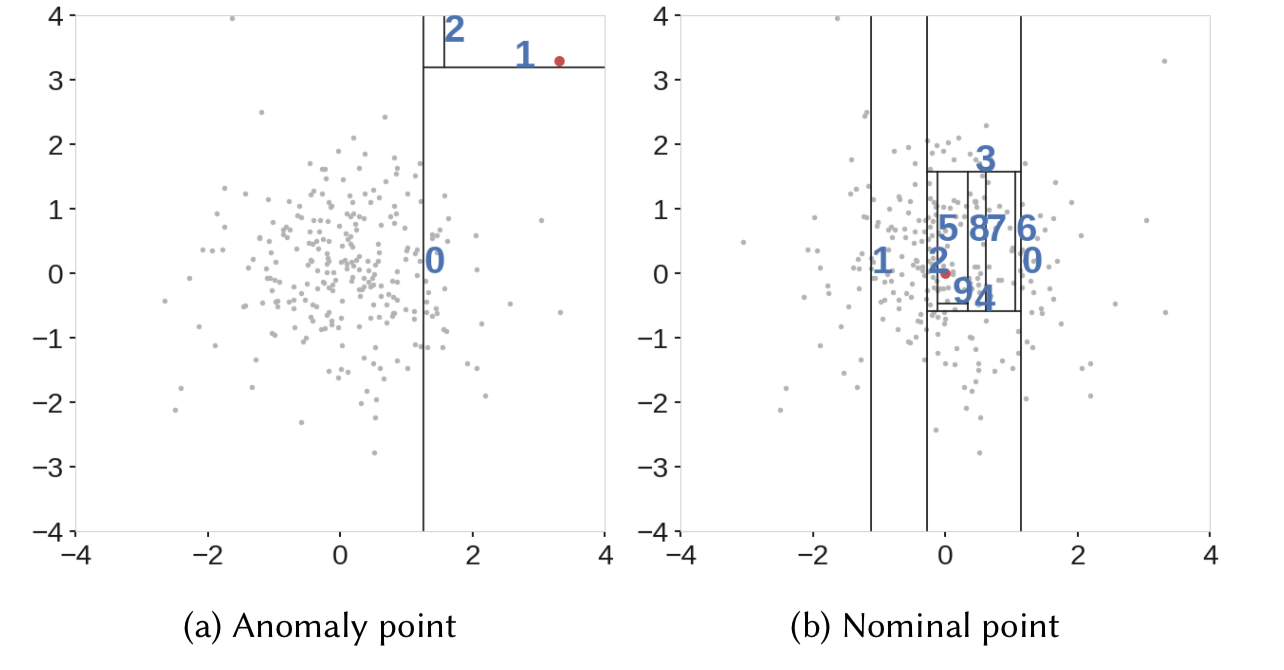
Source: IEEE. We can see that it was easier to isolate an anomaly compared to a normal observation.

Implementation in Python

Let us look at how to implement Isolation Forest in Python.

Step1: Read the Input Data

import numpy as np
import pandas as pd
import seaborn as sns
from sklearn.ensemble import IsolationForest
data = pd.read_csv('marks.csv')
data.head(10)

Output: 

Step2: Visualize the Data

From the box plot, we can infer that there are anomalies on the right.

Step3: Define and Fit the Model

random_state = np.random.RandomState(42)

model=IsolationForest(n_estimators=100,max_samples='auto',contamination=float(0.2),random_state=random_state)

model.fit(data[['marks']])

print(model.get_params())

Output:

{'bootstrap': False, 'contamination': 0.2, 'max_features': 1.0, 'max_samples': 'auto', 'n_estimators': 100, 'n_jobs': None, 'random_state': RandomState(MT19937) at 0x7F08CEA68940, 'verbose': 0, 'warm_start': False}

You can take a look at Isolation Forest documentation in sklearn to understand the model parameters.

Score the data to obtain anomaly scores:

data['scores'] = model.decision_function(data[['marks']])

data['anomaly_score'] = model.predict(data[['marks']])

data[data['anomaly_score']==-1].head()

Output:

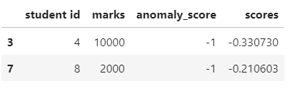
Here, we can observe that both anomalies are assigned an anomaly score of -1.

Step4: Model Evaluation

accuracy = 100*list(data['anomaly_score']).count(-1)/(anomaly_count)
print("Accuracy of the model:", accuracy)

Output:

Accuracy of the model: 100.0

What happens if we change the contamination parameter? Give it a try!!

Limitations of Isolation Forest

Isolation Forests are computationally efficient and researchers have proven them to be very effective in anomaly detection. Despite its advantages, there are a few limitations as mentioned below.

• The final anomaly score depends on the contamination parameter, provided while training the model. This implies that we should have an idea of what percentage of the data is anomalous beforehand to get a better prediction.
• Also, the model suffers from a bias due to the way the branching takes place.

Anomaly Score Map

Well, to understand the second point, we can take a look at the below anomaly score map.

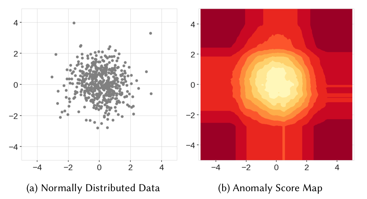
Source: IEEE

Here, in the score map on the right, we can observe that the points in the center obtained the lowest anomaly score, as expected. However, we can see four rectangular regions around the circle with lower anomaly scores as well. So, when scoring a new data point in any of these rectangular regions, it might not detect it as an anomaly.

Similarly, in the above figure, we can see that the model resulted in two additional blobs(on the top right and bottom left ) which never even existed in the data.

Whenever a node splits in an iTree based on a threshold value, it divides the data into left and right branches, resulting in horizontal and vertical branch cuts. And these branch cuts result in this model bias.

Result

The above figure shows branch cuts after combining outputs of all the trees of an Isolation Forest. Here, we can observe how the rectangular regions with lower anomaly scores formed in the left figure. And also the right figure shows the formation of two additional blobs due to more branch cuts.

To overcome this limit, an extension to Isolation Forests called ‘Extended Isolation Forests’ was introduced by Sahand Hariri. In EIF, horizontal and vertical cuts were replaced with cuts with random slopes.

Despite introducing EIF (Extended Isolation Forest), the use of Isolation Forests for anomaly detection remains widespread across various fields.

Conclusion

The Local Outlier Factor (LOF) algorithm is a powerful tool for detecting anomalies in data by evaluating the density of points relative to their neighbors. Unlike traditional anomaly detection methods, LOF does not require assuming a specific data distribution, making it suitable for a wide range of applications. When implementing LOF, setting the n_estimators parameter appropriately ensures robust performance, balancing computational efficiency with detection accuracy. It is important to note that LOF performs well with both normal and anomalous instances, as it identifies points that deviate significantly from their local neighborhood.

By leveraging random partitioning and regression techniques, LOF achieves scalable and efficient anomaly detection, even with large datasets. Adjusting the sampling size parameter enables fine-tuning of the algorithm to suit specific data characteristics, ensuring optimal results in real-world applications.

Key Takeaways

• ACM is a premier organization that provides resources and promotes research in computer science and information technology.
• An important challenge in data analysis, high-dimensional data refers to datasets with a large number of variables, which can complicate analysis and interpretation.
• In data structures like graphs, finding shorter paths is crucial for optimizing algorithms such as Dijkstra’s algorithm for pathfinding in graphs.
• In data analysis, analysts use a subset as a portion of a larger set to focus on specific parts of the data that are relevant to a particular question or analysis.
• Time series data analysts analyze observations collected at regular time intervals to extract meaningful insights or forecast future values.
• A potential reference that could be related to a person, place, or specific context not fully clear from the request.
• In machine learning, we use training data to build and train models, which then make predictions on new data.
• Normal data serves as a baseline for identifying anomalies or unusual occurrences within a dataset.

Frequently Asked Questions

The media shown in this article are not owned by Analytics Vidhya and are used at the Author’s discretion.