Gradient Boosting Algorithm: A Complete Guide for Beginners

Introduction

Prediction models are one of the most commonly used machine learning models. Gradient boosting is a method standing out for its prediction speed and accuracy, particularly with large and complex datasets. From Kaggle competitions to machine learning solutions for business, this algorithm has produced the best results. It is a boosting method and I have talked more about boosting in this article. It is more popularly known as Gradient Boosting Machine or GBM. In this article, I am going to discuss the math intuition behind the Gradient boosting algorithm.

This article was published as a part of the Data Science Blogathon

What is Boosting?

While studying machine learning you must have come across this term called boosting. It is the most misinterpreted term in the field of Data Science. The principle behind boosting algorithms is first we build a model on the training dataset, then a second model is built to rectify the errors present in the first model. Let me try to explain to you what exactly this means and how this works.

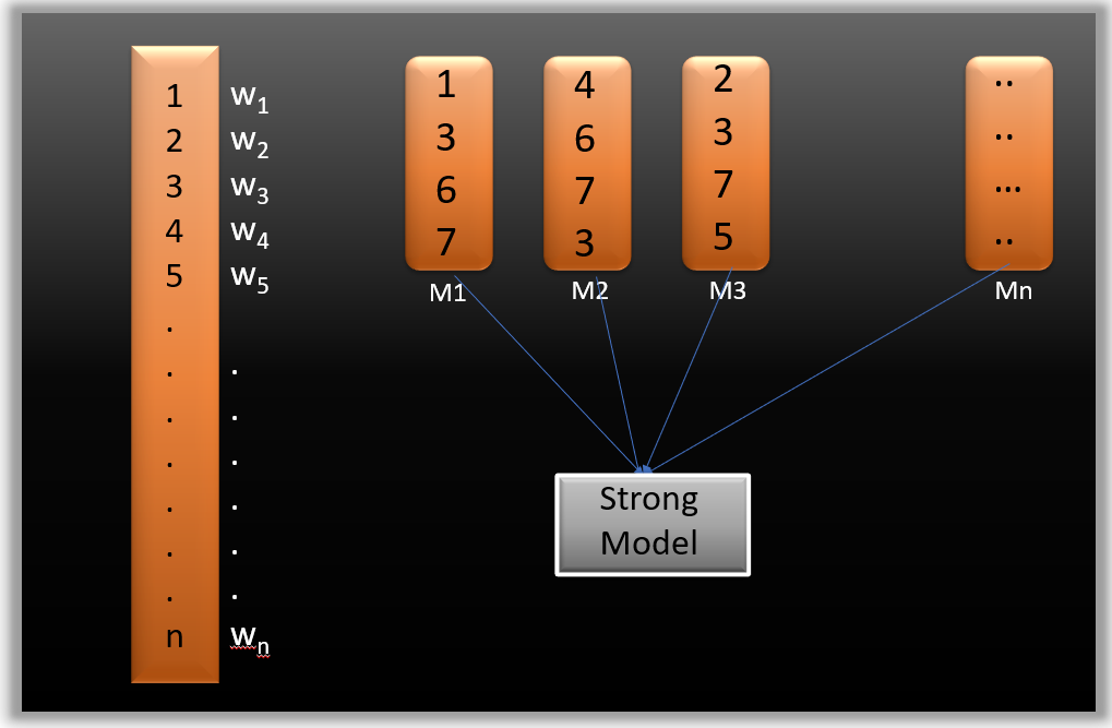
Suppose you have n data points and 2 output classes (0 and 1). You want to create a model to detect the class of the test data. Now what we do is randomly select observations from the training dataset and feed them to model 1 (M1), we also assume that initially, all the observations have an equal weight which means an equal probability of getting selected.

Remember in ensembling techniques the weak learners combine to make a strong model so here M1, M2, M3….Mn, are all weak learners.

Since M1 is a weak learner, it will surely misclassify some of the observations. Now, before feeding the observations to M2, we update the weights of the observations which are wrongly classified. You can think of it as a bag that initially contains 10 different color balls, but after some time, some kid takes out his favorite color ball and puts 4 red color balls instead inside the bag. Now, of course, the probability of selecting a red ball is higher.

Other Gradient Boosting Techniques

This same phenomenon happens in gradient boosting techniques, when an observation is wrongly classified, its weight gets updated, and for those which are correctly classified, their weights get decreased. The probability of selecting a wrongly classified observation increases. Hence, in the next model, only those observations get selected that were misclassified in model 1.

Similarly, it happens with M2, the wrongly classified weights are again updated and then fed to M3. This procedure is continued until and unless the errors are minimized, and the dataset is predicted correctly. Now when the new datapoint comes in (Test data) it passes through all the models (weak learners) and the class that gets the highest vote is the output for our test data.

What is Gradient Boosting?

Gradient boosting is a machine learning ensemble technique that combines the predictions of multiple weak learners, typically decision trees, sequentially. It aims to improve overall predictive performance by optimizing the model’s weights based on the errors of previous iterations, gradually reducing prediction errors and enhancing the model’s accuracy. This is most commonly used for linear regression.

What is AdaBoost Algorithm?

Before getting into the details of the gradient boosting algorithm, we must have some knowledge about the AdaBoost Algorithm which is again a boosting method. This algorithm starts by building a decision stump and then assigning equal weights to all the data points. Then it increases the weights for all the points that are misclassified and lowers the weight for those that are easy to classify or are correctly classified. A new decision stump is made for these weighted data points. The idea behind this is to improve the predictions made by the first stump. I have talked more about this algorithm here. Read this article before starting this algorithm to get a better understanding.

The main difference between these two algorithms is that gradient boosting has a fixed base estimator i.e., decision trees whereas in AdaBoost we can change the base estimator according to our needs.

What is a Gradient Boosting Algorithm?

Errors play a major role in any machine learning algorithm. There are mainly two types of errors: bias error and variance error. The gradient boost algorithm helps us minimize the bias error of the model. The main idea behind this algorithm is to build models sequentially and these subsequent models try to reduce the errors of the previous model. But how do we do that? How do we reduce the error? This is done by building a new model on the errors or residuals of the previous model.

When the target column is continuous, we use Gradient Boosting Regressor whereas when it is a classification problem, we use Gradient Boosting Classifier. The only difference between the two is the “Loss function”. The objective here is to minimize this loss function by adding weak learners using gradient descent. Since it is based on the++ loss function, for regression problems, we’ll have different loss functions like Mean squared error (MSE) and for classification, we will have different functions, like log-likelihood.

Understanding Gradient Boosting Algorithm with An Example

Let’s understand the intuition behind the gradient boosting algorithm with the help of an example. Here our target column is continuous hence we will use gradient boosting regressor.

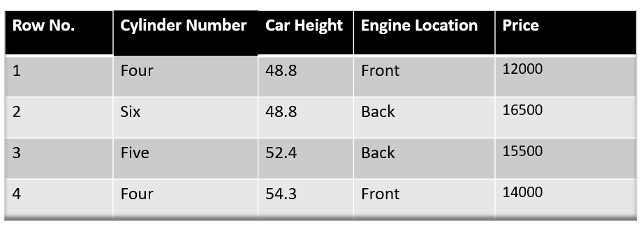
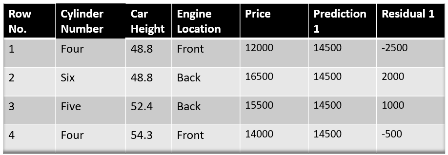
Following is a sample from a random dataset where we have to predict the car price based on various features. The target column is price and other features are independent features.

Step 1: Build a Base Model

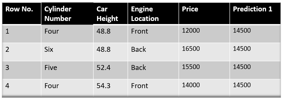
The first step in gradient boosting is to build a base model to predict the observations in the training dataset. For simplicity, we take an average of the target column and assume that to be the predicted value as shown below:

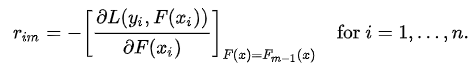
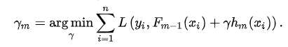
Why did I say we take the average of the target column? Well, there is math involved in this. Mathematically the first step can be written as:

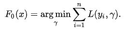
Looking at this may give you a headache, but don’t worry we will try to understand what is written here.

Here L is our loss function,
Gamma is our predicted value, and
arg min means we have to find a predicted value/gamma for which the loss function is minimum.

Since the target column is continuous our loss function will be:

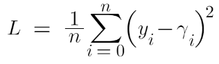
Here y_i is the observed value, and gamma is the predicted value.

Now we need to find a minimum value of gamma such that this loss function is minimum. We all have studied how to find minima and maxima in our 12th grade. Did we use it to differentiate this loss function and then put it equal to 0 right? Yes, we will do the same here.

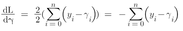
Let’s see how to do this with the help of our example. Remember that y_i is our observed value and gamma_i is our predicted value, by plugging the values in the above formula we get:

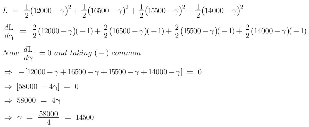
We end up over an average of the observed car price and this is why I asked you to take the average of the target column and assume it to be your first prediction.

Hence for gamma=14500, the loss function will be minimum so this value will become our prediction for the base model.

Step 2: Compute Pseudo Residuals

The next step is to calculate the pseudo residuals which are (observed value – predicted value).

Again the question comes why only observed – predicted? Everything is mathematically proven. Let’s see where this formula comes from. This step can be written as:

Here F(x_i) is the previous model and m is the number of DT made.

We are just taking the derivative of loss function w.r.t the predicted value and we have already calculated this derivative:

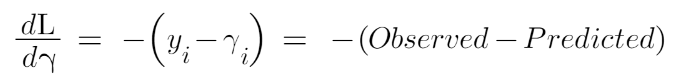
If you see the formula of residuals above, we see that the derivative of the loss function is multiplied by a negative sign, so now we get:

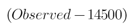
The predicted value here is the prediction made by the previous model. In our example the prediction made by the previous model (initial base model prediction) is 14500, to calculate the residuals our formula becomes:

Step 3: Build a Model on Calculated Residuals

In the next step, we will build a model on these pseudo residuals and make predictions. Why do we do this? Because we want to minimize these residuals minimizing the residuals will eventually improve our model accuracy and prediction power. So, using the Residual as a target and the original feature Cylinder number, cylinder height, and Engine location we will generate new predictions. Note that the predictions, in this case, will be the error values, not the predicted car price values since our target column is an error now.

Let’s say h_m(x) is our DT made on these residuals.

Step 4: Compute Decision Tree Output

In this step, we find the output values for each leaf of our decision tree. That means there might be a case where 1 leaf gets more than 1 residual, hence we need to find the final output of all the leaves. To find the output we can simply take the average of all the numbers in a leaf, doesn’t matter if there is only 1 number or more than 1.

Let’s see why we take the average of all the numbers. Mathematically this step can be represented as:

Here h_m(x_i) is the DT made on residuals and m is the number of DT. When m=1 we are talking about the 1st DT and when it is “M” we are talking about the last DT.

The output value for the leaf is the value of gamma that minimizes the Loss function. The left-hand side “Gamma” is the output value of a particular leaf. On the right-hand side [F m-1 (x i )+ƴh m (x i ))] is similar to step 1 but here the difference is that we are taking previous predictions whereas earlier there was no previous prediction.

Example of Calculating Regression Tree Output

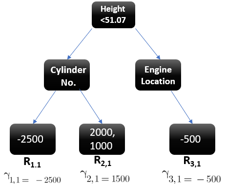
Let’s understand this even better with the help of an example. Suppose this is our regressor tree:

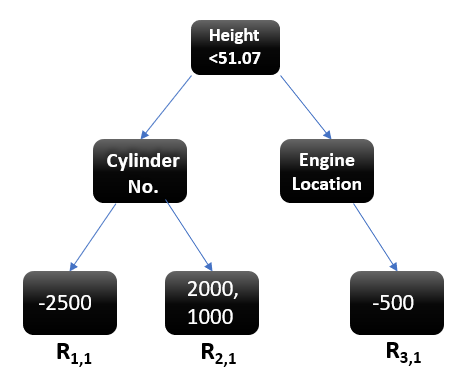
We see 1^st residual goes in R_1,1  ,2^nd and 3^rd residuals go in R_2,1 and 4^th residual goes in R_3,1 .

Let’s calculate the output for the first leave that is R_1,1

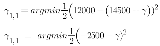
Now we need to find the value for gamma for which this function is minimum. So we find the derivative of this equation w.r.t gamma and put it equal to 0.

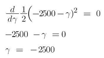
Hence the leaf R_1,1 has an output value of -2500. Now let’s solve for the R_2,1.

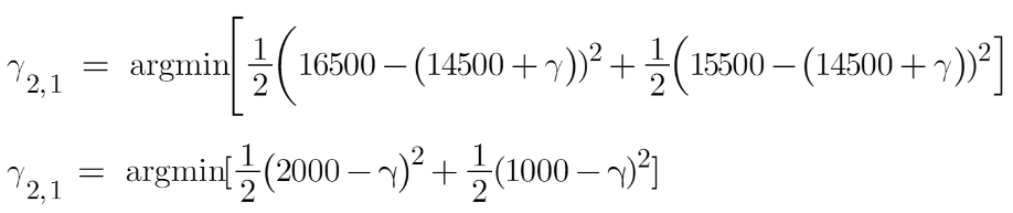
Let’s take the derivative to get the minimum value of gamma for which this function is minimum:

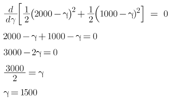
We end up with the average of the residuals in the leaf R_2,1 . Hence if we get any leaf with more than 1 residual, we can simply find the average of that leaf and that will be our final output.

Now after calculating the output of all the leaves, we get:

Step 5: Update Previous Model Predictions

This is finally the last step where we have to update the predictions of the previous model. It can be updated as:

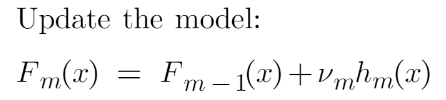
where m is the number of decision trees made.

Since we have just started building our model so our m=1. Now to make a new DT our new predictions will be:

Here F_m-1(x) is the prediction of the base model (previous prediction) since F_1-1=0 , F₀ is our base model hence the previous prediction is 14500.

nu is the learning rate that is usually selected between 0-1. It reduces the effect each tree has on the final prediction, and this improves accuracy in the long run. Let’s take nu=0.1 in this example.

H_m(x) is the recent DT made on the residuals.

Let’s calculate the new prediction now:

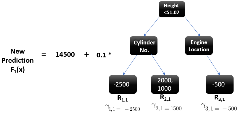
Suppose we want to find a prediction of our first data point which has a car height of 48.8. This data point will go through this decision tree and the output it gets will be multiplied by the learning rate and then added to the previous prediction.

Now let’s say m=2 which means we have built 2 decision trees and now we want to have new predictions.

This time we will add the previous prediction that is F₁(x) to the new DT made on residuals. We will iterate through these steps again and again till the loss is negligible.

I am taking a hypothetical example here just to
make you understand how this predicts for a new dataset:

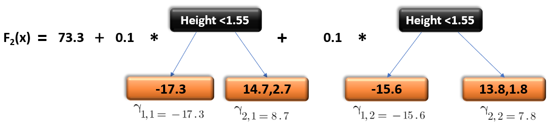
If a new data point comes, say, height = 1.40, it’ll go through all the trees and then will give the prediction. Here we have only 2 trees hence the datapoint will go through these 2 trees and the final output will be F₂(x).

What is a Gradient Boosting Classifier?

A gradient-boosting classifier is used when the target column is binary. All the steps explained in the gradient boosting regressor are used here, the only difference is we change the loss function. Earlier we used Mean squared error when the target column was continuous but this time, we will use log-likelihood as our loss function.

Let’s see how this loss function works, to read more about log-likelihood I recommend you to go through this article where I have given each detail you need to understand this.

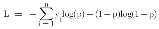
The loss function for the classification problem is given below:

Our first step in the gradient boosting algorithm was to initialize the model with some constant value, there we used the average of the target column but here we’ll use log(odds) to get that constant value. The question comes why log(odds)?

When we differentiate this loss function, we will get a function of log(odds) and then we need to find a value of log(odds) for which the loss function is minimum.

How Does it Work?

Are you confused right? now Okay let’s see how it works:

Let’s first transform this loss function so that it is a function of log(odds), I’ll tell you later why we did this transformation.

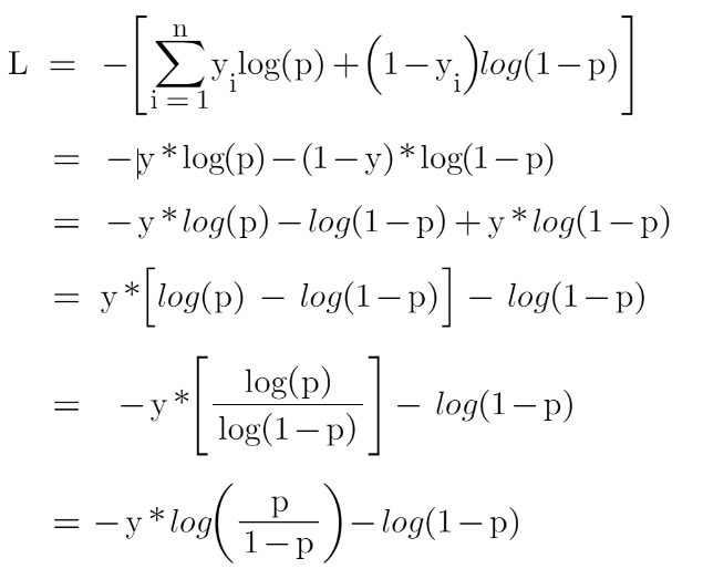
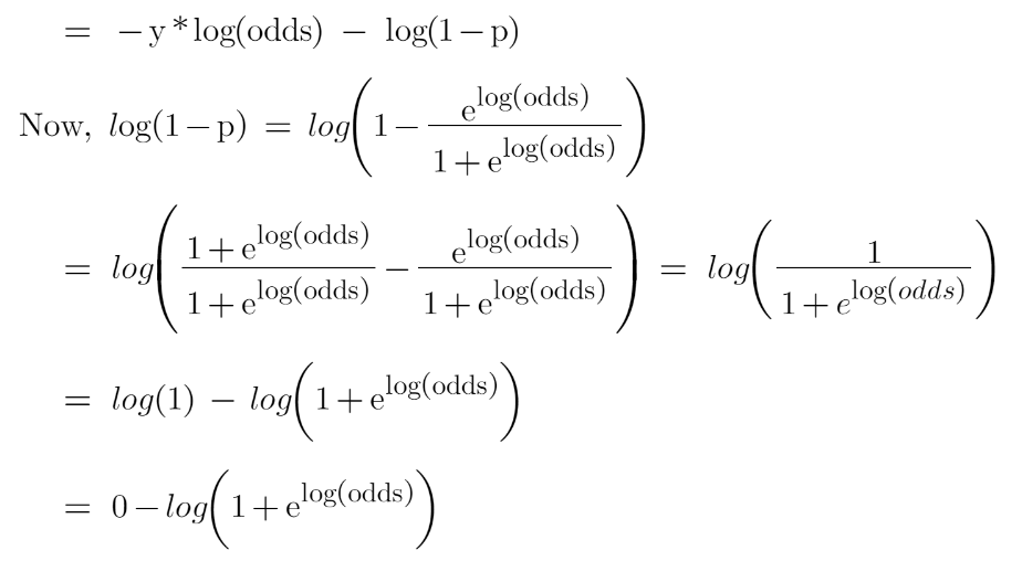
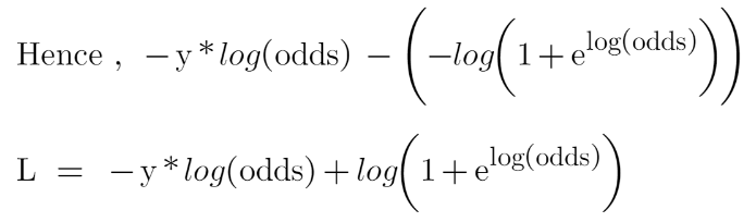
Now this is our loss function, and we need to minimize it, for this, we take the derivative of this w.r.t to log(odds) and then put it equal to 0,

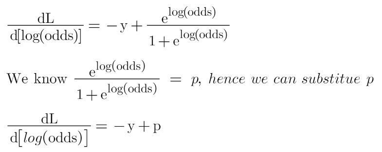
Here, ‘y’ denotes the observed values.

You must be wondering why we transformed the loss function into a function of log(odds). Sometimes it is easy to use the function of log(odds), and sometimes it’s easy to use the function of predicted probability “p”.

It isn’t compulsory to transform the loss function, we did this just to have easy calculations.

Hence the minimum value of this loss function will be our first prediction (base model prediction)

Now in the gradient boosting regressor, our next step was to calculate the pseudo residuals where we multiplied the derivative of the loss function with -1. We will do the same but now the loss function is different, and we are dealing with the probability of an outcome now.

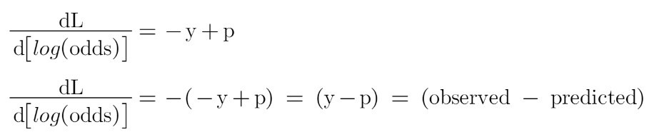
After finding the residuals we can build a decision tree with all independent variables and target variables as “Residuals”.

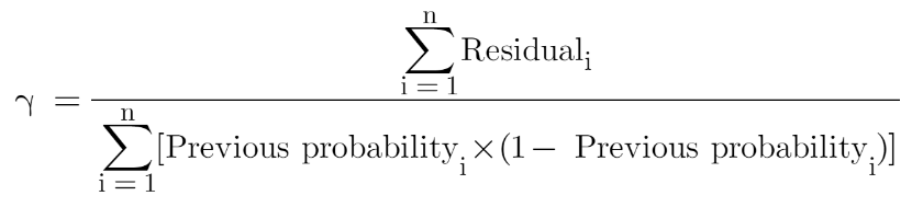
Now when we have our first decision tree, we find the final output of the leaves because there might be a case where a leaf gets more than 1 residuals, so we need to calculate the final output value. The math behind this step is out of the scope of this article so I will mention the direct formula to calculate the output of a leaf:

Finally, we are ready to get new predictions by adding our base model with the new tree we made on residuals.

Implementation of GBM Using scikit-learn

For the implementation of GBM on a dataset, we will be using the Income Evaluation dataset, which has information about an individual’s personal life and an output of 50K or <=50. The dataset can be found here (https://www.kaggle.com/lodetomasi1995/income-classification)

The task here is to classify the income of an individual when given the required inputs about his personal life.

First, let’s import all required libraries.

# Import all relevant libraries

from sklearn.ensemble import GradientBoostingClassifier

import numpy as np

import pandas as pd

from sklearn.preprocessing import StandardScaler

from sklearn.model_selection import train_test_split

from sklearn.metrics import accuracy_score, confusion_matrix

from sklearn import preprocessing

import warnings

warnings.filterwarnings("ignore")

Now let’s read the dataset and look at the columns to understand the information better.

df = pd.read_csv('income_evaluation.csv')
df.head()

I have already done the data preprocessing part and you can see the whole code here. Here my main aim is to tell you how to implement this in Python. Now for training and testing our model, the data has to be divided into train and test sets.

We will also scale the data to lie between 0 and 1.

# Split dataset into test and train data

X_train, X_test, y_train, y_test = train_test_split(df.drop(‘income’, axis=1),df[‘income’], test_size=0.2)

Now let’s go ahead with defining the Gradient Boosting Classifier along with its hyperparameters. Next, we will fit this model into the training data.

# Define Gradient Boosting Classifier with hyperparameters

gbc=GradientBoostingClassifier(n_estimators=500,learning_rate=0.05,random_state=100,max_features=5 )

# Fit train data to GBC

gbc.fit(X_train,y_train)

The model has been trained and we can now observe the outputs as well.

Below, you can see the confusion matrix of the model, which gives a report of the number of classifications and misclassifications.

# Confusion matrix will give number of correct and incorrect classifications
print(confusion_matrix(y_test, gbc.predict(X_test)))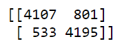

The number of misclassifications by the Gradient Boosting Classifier is 1334, compared to 8302 correct classifications. The model has performed decently.
Let’s check the accuracy:

# Accuracy of model

print("GBC accuracy is %2.2f" % accuracy_score( 
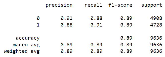
     y_test, gbc.predict(X_test)))

Let’s check the classification report also:

from sklearn.metrics import classification_report 

pred=gbc.predict(X_test) 

print(classification_report(y_test, pred))

The accuracy is 86%, which is pretty good but this can be improved by tuning the hyperparameters or processing the data to remove outliers.
This however gives us the basic idea behind gradient boosting and its underlying working principles.

The accuracy is 86%, which is pretty good but this can be improved by tuning the hyperparameters or processing the data to remove outliers.
This however gives us the basic idea behind gradient boosting and its underlying working principles.

Parameter Tuning in Gradient Boosting (GBM) in Python

Tuning n_estimators and Learning rate

n_estimators is the number of trees (weak learners) that we want to add in the model. There are no optimum values for the learning rate as low values always work better, given that we train on a sufficient number of trees. A high number of trees can be computationally expensive. That’s why I have taken a few number of trees here.

from sklearn.model_selection import GridSearchCV

grid = {

    'learning_rate':[0.01,0.05,0.1],

    'n_estimators':np.arange(100,500,100),

}


gb = GradientBoostingClassifier()

gb_cv = GridSearchCV(gb, grid, cv = 4)

gb_cv.fit(X_train,y_train)

print("Best Parameters:",gb_cv.best_params_)

print("Train Score:",gb_cv.best_score_)

print("Test Score:",gb_cv.score(X_test,y_test))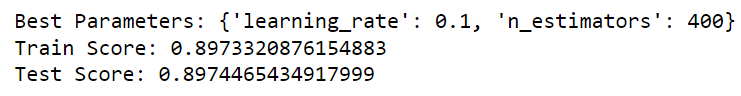

We see the accuracy increased from 86 to 89 after tuning n_estimators and learning rate. Also the “true positive” and the “true negative” rate improved.

We can also tune max_depth parameter which you must have heard in decision trees and random forests.

grid = {'max_depth':[2,3,4,5,6,7] }

gb = GradientBoostingClassifier(learning_rate=0.1,n_estimators=400)

gb_cv = GridSearchCV(gb, grid, cv = 4)

gb_cv.fit(X_train,y_train)

print("Best Parameters:",gb_cv.best_params_)

print("Train Score:",gb_cv.best_score_)

print("Test Score:",gb_cv.score(X_test,y_test))

The accuracy increased even more when we tuned the parameter “max_depth”.

Conclusion

I hope you got an understanding of how the Gradient Boosting algorithm works under the hood. I have tried to show you the math behind this in the easiest way possible. Apart from this, there are many other techniques for improving model performance, such as XGBoost, LightGBM, and CatBoost. I will explain about these in my upcoming articles.

Frequently Asked Questions

The media shown in this article are not owned by Analytics Vidhya and are used at the Author’s discretion.

Anshul Saini 25 May 2024

I am an undergraduate student currently in my last year majoring in Statistics (Bachelors of Statistics) and have a strong interest in the field of data science, machine learning, and artificial intelligence. I enjoy diving into data to discover trends and other valuable insights about the data. I am constantly learning and motivated to try new things.