The "Teacher’s Corner" of The American Statistician enables statisticians to discuss topics that are relevant to teaching and learning statistics. Sometimes, the articles have practical relevance, too. Andersson (2023) "The Wald Confidence Interval for a Binomial p as an Illuminating 'Bad' Example," is intended for professors and masters-level students in mathematical statistics. However, the topic has practical importance. The introduction to the article states, "the standard two-sided Wald interval for the binomial [proportion]is ... known to be of low quality with respect to actual coverage, and it ought to be stricken from all courses" in favor of alternative intervals such as the Wilson (score).
If Andersson wants the method "stricken from all courses," then presumably he also advocates that the Wald CI should not be used in practice. That is a strong statement with practical importance. The Wald confidence interval (CI) is the default CI for PROC FREQ in SAS, although the documentation states "the Wilson interval has ... better performance than the Wald interval."
Let's investigate this issue. This article presents a simulation study that compares the coverage probability of the two-sided CIs for the (uncorrected) Wald method and for the Wilson (score) method. The simulation demonstrates that Andersson makes an excellent point: In practice, the Wald method is an inferior choice for the CI. You can use the Wilson CI to obtain a better confidence interval. In PROC FREQ, you can use the BINOMIAL(CL=WILSON) option on the TABLES statement to obtain the Wilson CI.
The Wald confidence interval for a binomial proportion
As Andersson (2023) points out, "generations" of students have memorized the formula for the Wald CI, "and probably some of them still remember it."
If a sample has n observations and n1 are an event of interest, then
a point-estimate for the proportion of events is \(\hat{p} = n_1 / n\). This is called "the binomial proportion" because the distribution of n1 is Binomial(p, n).
The Wald confidence interval for the proportion is given by the formula
\(
\hat{p} \pm z \sqrt { \hat{p} (1 - \hat{p} ) / n }
\)
where z is the (1-α/2)th quantile of the standard normal distribution.
The formula for the Wilson interval is given in the documentation of PROC FREQ.
I won't repeat Andersson's mathematical arguments about why the Wald interval is deficient, but a few issues are:
- The point estimator and its standard error (the quantity under the square root sign) are correlated.
- The Wald CI approximates the discrete sampling distribution of the Wald statistic by using a continuous normal distribution. This leads to a mismatch between the quantiles of the actual sampling distribution and the approximate quantiles.
- The Wald statistic is biased, skewed, and exhibits excess kurtosis. (See Table 1 in Andersson (2023).)
- The Wald interval has lower-than-expected coverage. For example, a 95% confidence interval might contain the proportion parameter for only 93% of random samples.
Coverage probability for the Wald confidence interval
Andersson states that the Wald interval is "low quality with respect to actual coverage." The coverage probability of a confidence interval is the probability that the interval (which is a statistic) contains the value of the distribution parameter. For example, a 95% confidence interval should contain the distribution parameter in 95% of all random samples. For the binomial proportion, you can run a simulation to estimate the coverage probability of the Wald interval and Wilson intervals, as follows:
- Choose a proportion parameter, p.
- Simulate n independent Bernoulli trials with probability p. This results in n1 events. Equivalently, yhat you can simulate the n1 values directly from the Binomial(p, n) distribution.
- Calculate the Wald and Wilson intervals. Assess whether the parameter is inside each interval.
- Repeat the simulation B times, where B is a large number. Estimate the coverage probability as k/B, where k is the number of times that the parameter is in the confidence interval.
The following SAS program simulates B=10,000 samples of size n=50 from the Binomial(p, n) distribution for p=0.2. You can use PROC FREQ to estimate the proportion and confidence intervals from each sample. The OUTPUT statement writes the statistics to a SAS data set. The variables L_Bin and U_Bin are the lower and upper confidence limits, respectively, for the Wald interval. The variables L_W_Bin and U_W_Bin are the corresponding limits for the Wilson interval. A second DATA step creates binary variables that indicate whether each interval contains the parameter, p. A second call to PROC FREQ calculates the proportion of samples for which the interval contains the parameter, which estimates the coverage probability.
/* simulation of Wald interval vs Wilson interval for binomial proportion */ %let B = 10000; /* number of simulations in study */ %let N = 50; /* sample size */ data BinomSim; call streaminit(12345); N = &N; do p = 0.2; do ID = 1 to &B; Event = 1; Count = rand("Binom", p, N); /* number of events in N trials */ output; Event = 0; Count = N - Count; /* number of non-events */ output; end; end; run; /* for each sample, estimate proportion and CIs (Wald and Wilson) */ proc freq data=BinomSim noprint; by p ID; weight Count / zeros; tables Event / nocum binomial(level='1' CL=Wald CL=Wilson); output out=Est binomial; run; /* create binary (0/1) variables that indicate whether p is in the CI */ data Coverage; set Est; label _BIN_="Estimate (pHat)" L_Bin="Lower Wald CL" U_Bin="Upper Wald CL" L_W_Bin="Lower Wilson CL" U_W_Bin="Upper Wilson CL"; WaldInCL = (L_Bin <= p & p <= U_Bin); /* is p in Wald CI? */ WilsonInCL = (L_W_Bin <= p & p <= U_W_Bin); /* is p in Wilson CI? */ keep p ID _Bin_ L_Bin U_Bin L_W_Bin U_W_Bin WaldInCL WilsonInCL; run; /* estimate the empirical coverage probability for the nominal 95% CIs */ proc freq data=Coverage; by p; tables WaldInCL WilsonInCl / nocum; run; |
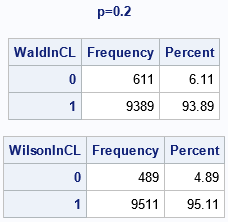
The output for p=0.2 is shown. We wanted 95% confidence intervals, but the simulation p indicates that the empirical coverage probability for the Wald confidence interval is about 93.89%, which is substantially lower than 95%. In contrast, the empirical coverage probability for the Wald confidence interval is about 95.11% when p=0.2.
Repeat the simulation for a range of parameters
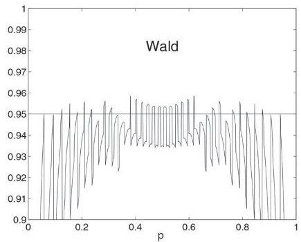
Andersson's article taught me something new. Namely, that the coverage probability for an interval is not a smooth (or even continuous) function of the proportion parameter. I knew that interval estimates are better when p ≈ 1/2 and can be bad when p is near 0 or 1, but I did not know that the coverage probability can jump dramatically if you change p by a small amount. Andersson shows this in Figure 1, which is reproduced on the right. Andersson states that "the ragged performance" is "due to the lattice structure of the binomial distribution." This phenomenon is explained in Brown, Cai, and DasGupta (2001), which contains several similar plots. The phenomenon is not some artifact of the Wald interval. It is a real phenomenon that affects all confidence intervals, including the Wilson interval.
Let's extend the simulation so that it estimates the Wald and Wilson coverage probability for a range of proportion parameters. Most textbooks caution that you should not use the Wald interval unless np(1-p) > 5, which means that when n=50 we should consider only p > 0.11. You can convert the previous simulation to a series of simulations by changing one line in the first DATA step. You should replace the line that sets p=0.2 with a DO loop that iterates over a range of values.
/* simulation of Wald interval vs Wilson interval for binomial proportion */ %let B = 10000; /* number of simulations in study */ %let N = 50; /* sample size */ /* Simulate random samples of size N where Pr(Event=1)=p */ data BinomSim; call streaminit(12345); N = &N; /* n*p*(1-p) > 5 ==> p > 0.1127 */ do p = 0.11 to 0.5 by 0.005; /* <== iterate over a range of proportion parameters */ do ID = 1 to &B; Event = 1; Count = rand("Binom", p, N); /* number of events in N trials */ output; Event = 0; Count = N - Count; /* number of non-events */ output; end; end; run; /* construct Wald and Wilson CIs for estimate of proportion, \hat{p} */ proc freq data=BinomSim noprint; by p ID; weight Count / zeros; tables Event / nocum binomial(level='1' CL=Wald CL=Wilson); output out=Est binomial; run; /* create binary variable to indicate whether interval contains p */ data Coverage; set Est; label _BIN_="Estimate (pHat)" L_Bin="Lower Wald CL" U_Bin="Upper Wald CL" L_W_Bin="Lower Wilson CL" U_W_Bin="Upper Wilson CL"; WaldInCL = (L_Bin <= p & p <= U_Bin); /* is p in Wald CI? */ WilsonInCL = (L_W_Bin <= p & p <= U_W_Bin); /* is p in Wilson CI? */ keep p ID _Bin_ L_Bin U_Bin L_W_Bin U_W_Bin WaldInCL WilsonInCL; run; |
Instead of looking at tables of the empirical coverage probabilities, the following program statements graph the estimated coverage versus the parameter for both the Wald and Wilson intervals:
/* plot empirical coverage probability of the Wald CI for range of p */ proc freq data=Coverage noprint; by p; tables WaldInCL / nocum binomial(level='1' CL=Wilson); output out=CoverageWard binomial; run; title "Coverage Probability of Ward CI"; proc sgplot data=CoverageWard; label _BIN_="Ward Coverage" p="Binomial Probability"; scatter y=p x=_BIN_ / xerrorlower=L_W_Bin xerrorupper=U_W_Bin; refline 0.95 / axis=x noclip; xaxis min=0.88 max=0.98; run; /* plot empirical coverage probability of the Wilson CI for range of p */ proc freq data=Coverage noprint; by p; tables WilsonInCL / nocum binomial(level='1' CL=Wilson); output out=CoverageWilson binomial; run; title "Coverage Probability of Wilson CI"; proc sgplot data=CoverageWilson; label _BIN_="Wilson Coverage" p="Binomial Probability"; scatter y=p x=_BIN_ / xerrorlower=L_W_Bin xerrorupper=U_W_Bin; refline 0.95 / axis=x noclip; xaxis min=0.88 max=0.98; run; |

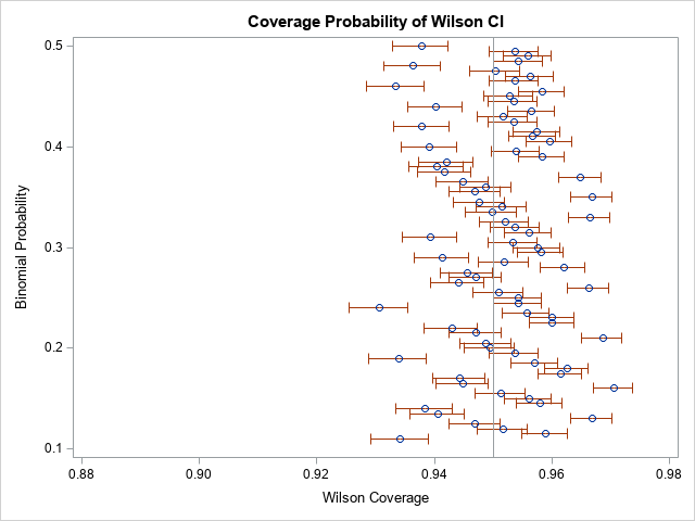
I've aligned the graphs for comparison. From the graphs, you can notice the following:
- The coverage probability "jumps around" in both graphs as the parameter, p, changes. This is a real phenomenon and is not due to Monte Carlo variation.
- In general, the Wald confidence interval exhibits less than 95% coverage. For proportion parameters less than 0.2, the coverage is especially bad.
- Sometimes the Wilson confidence interval is less than 95% coverage, but other times it is more. The Wilson intervals appear to be roughly symmetric around the 95% reference line. This is a good property to have, as opposed to the systematic downward bias of the Wald CI.
These graphs show why the Wilson interval is preferred over the Wald interval. The Wald interval has actual coverage that is less than its nominal coverage. If you do not know the proportion parameter (and you never do!) then the Wilson interval is a more reliable and dependable interval. If you pardon the pun, you can have more "confidence" in the Wilson interval.
Summary
Andersson (2023) states, "the standard two-sided Wald interval for the binomial [proportion]is ... known to be of low quality with respect to actual coverage." The documentation for PROC FREQ in SAS agrees by stating, "the Wilson interval has ... better performance than the Wald interval." This article runs a simulation study that provides evidence for those statements.
Andersson suggests that the Wald CI should not be used in practice. In PROC FREQ in SAS, you can use the BINOMIAL(CL=WILSON) option on the TABLES statement to obtain the Wilson CI. With this small change to your programs, you will obtain a more reliable interval estimate for a binomial proportion.

3 Comments
Rick,
Interesting thing is EXACT CI would get different result.
Which would get reversed result with WALD .
tables Event / nocum binomial(level='1' CL=Wald CL=exact);
Thanks for writing. The CL=EXACT method produces the Clopper-Pearson CI, which uses probabilities from the discrete binomial distribution. The doc for PROC FREQ states:
"The confidence coefficient (coverage probability) of the exact (Clopper-Pearson) interval is not exactly (1 - α) but is at least (1 - α). Thus, this confidence interval is conservative. Unless the sample size is large, the actual coverage probability can be much larger than the target value."
Pingback: Estimate a proportion and a confidence interval in SAS - The DO Loop